Scilab @ ICATT 2016 --> Orbit Simulation Tutorial
Following the advice of our long-time partners from the French Space Agency CNES, we are presenting today at the 6th International Conference on Astrodynamics Tools and Techniques (ICATT).
To demonstrate the capacities of Scilab in this field, here is a classical problem of space mechanics solved step-by-step:
Satellite orbit around the earth
Download the script:
myEarthRotation.sci 1.77 kB
Download the full tutorial:
Scilab Orbite Simulation.pdf 1.35 MB
1. Express the physics problem
The problem is based on the universal law of gravitation:
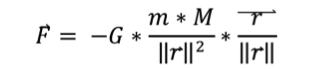
We write down Newton’s third law of motion in an earth-centred referential:
(1)
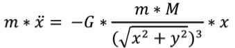
(2)
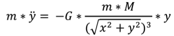
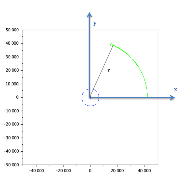
Position of the satellite is at a distance r [x; y]
Earth mass centre is at O [0; 0]
Gravitational constant:
![]()
Mass of the earth:
![]()
Radius of the Earth:
![]()
2. Translate your problem into Scilab
Scilab is a matrix-based language. Instead of expressing the system as set of 4 independent equations (along the x and y axis, for position and speed), we describe it as a single matrix equation, of dimension 4x4:
This method is a classical trick to switch from a second order scalar differential equation to a first order matrix differential equation.
![]()
with
To simplify the equation, we define the variable:
![]()
Open scinotes with edit myEarthRotation.sci
Define the skeleton of the function:
function U=earthrotation(altitude, v_init, hours)
// altitude given in km
// v_init is a vector [vx; vy] given in m/s
// hours is the number of hours for the simulation
r_earth = 6.378E6;
altitude = altitude * 1000;
U0 = [r_earth + altitude; 0; 0; v_init];
t = 0:10:(3600*hours); // simulation time, one point every 10 seconds
U = ode(U0, 0, t, f);

// Draw the earth in blue
angle = 0:0.01:2*%pi;
x_earth = 6378 * cos(angle);
y_earth = 6378 * sin(angle);
fig = scf();
a = gca();
a.isoview = "on";
plot(x_earth, y_earth, 'b--');
plot(0, 0, 'b+');

// Draw the trajectory computed
comet(U(1,:)/1000, U(2,:)/1000, "colors", 3);
endfunction
The condition defined by the distance r of the satellite with the centre of earth stops the simulation if it’s colliding with earth’s surface.
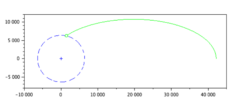
Try out the final script with the following initial conditions in speed and altitude:
--> geo_alt = 35784; // in kms
--> geo_speed = 1074; // in m/s
--> simulation_time = 24; // in hours
--> U = earthrotation(geo_alt, geo_speed, simulation_time);
3. Compute the results and create a visual animation
With this function, we go to the core of the problem:
function U=earthrotation(altitude, v_init, hours)
// altitude given in km
// v_init is a vector [vx; vy] given in m/s
// hours is the number of hours for the simulation
r_earth = 6.378E6;
altitude = altitude * 1000;
U0 = [r_earth + altitude; 0; 0; v_init];
t = 0:10:(3600*hours); // simulation time, one point every 10 seconds
U = ode(U0, 0, t, f);

// Draw the earth in blue
angle = 0:0.01:2*%pi;
x_earth = 6378 * cos(angle);
y_earth = 6378 * sin(angle);
fig = scf();
a = gca();
a.isoview = "on";
plot(x_earth, y_earth, 'b--');
plot(0, 0, 'b+');

// Draw the trajectory computed
comet(U(1,:)/1000, U(2,:)/1000, "colors", 3);
endfunction
The resolution of the ordinary differential equation (ODE) is computed with the Scilab function ode.
ode solves Ordinary Different Equations defined by:
![]()
where y is a real vector or matrix
The simplest call of ode is: y = ode(y0,t0,t,f) where y0 is the vector of initial conditions, t0 is the initial time, t is the vector of times at which the solution y is computed and y is matrix of solution vectors y=[y(t(1)),y(t(2)),...].
Go further
To go further in numerical analysis, find out more about the solvers:
Ordinary Differential Equations with Scilab, WATS Lectures, Université de Saint-Louis, G. Sallet, 2004
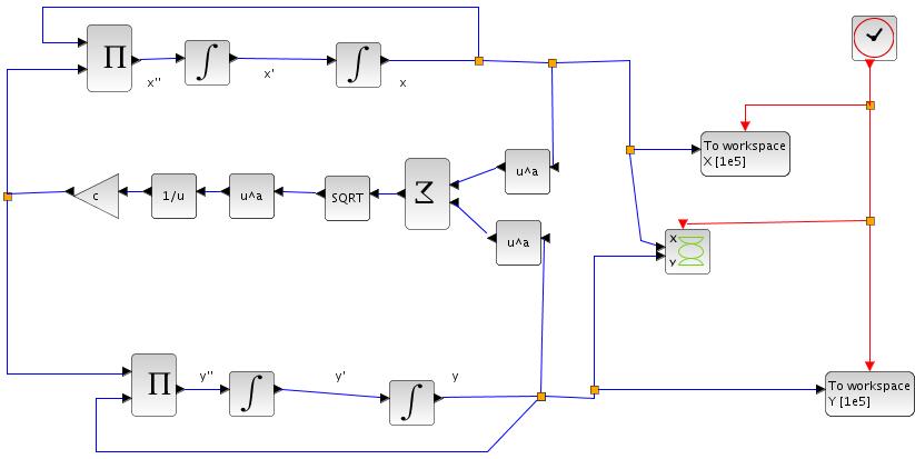
You can also model and simulate it with Xcos:
myEarthRotationXcos.zcos 6.99 kB