Machine learning – Logistic regression tutorial
Download this tutorial: doc or pdf
and the dataset: zip
—
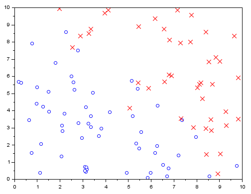
Let’s create some random data that are split into two different classes, ‘class 0’ and ‘class 1’.
We will use these data as a training set for logistic regression.
Import your data
This dataset represents 100 samples classified in two classes as 0 or 1 (stored in the third column), according to two parameters (stored in the first and second column):
data_classification.csv
Directly import your data in Scilab with the following command:
t=csvRead("data_classification.csv");
These data has been generated randomly by Scilab with the following script:
b0 = 10;
t = b0 * rand(100,2);
t = [t 0.5+0.5*sign(t(:,2)+t(:,1)-b0)];

b = 1;
flip = find(abs(t(:,2)+t(:,1)-b0))
The data from different classes overlap slightly. The degree of overlapping is controlled by the parameter b in the code.
Represent your data
Before representing your data, you need to split them into two classes t0 and t1 as followed:
t0 = t(find(t(:,$)==0),:);
t1 = t(find(t(:,$)==1),:);

clf(0);scf(0);
plot(t0(:,1),t0(:,2),'bo')
plot(t1(:,1),t1(:,2),'rx')
Build a classification model
We want to build a classification model that estimates the probability that a new, incoming data belong to the class 1.
First, we separate the data into features and results:
x = t(:, 1:$-1); y = t(:, $);

[m, n] = size(x);
Then, we add the intercept column to the feature matrix
// Add intercept term to x
x = [ones(m, 1) x];
The logistic regression hypothesis is defined as:
h(θ, x) = 1 / (1 + exp(−θTx) )
It’s value is the probability that the data with the features x belong to the class 1.
The cost function in logistic regression is
J = [−yT log(h) − (1−y)T log(1−h)]/m
where log is the “element-wise” logarithm, not a matrix logarithm.
Gradient descent
If we use the gradient descent algorithm, then the update rule for the θ is
θ → θ − α ∇J = θ − α xT (h − y) / m
The code is as follows
// Initialize fitting parameters
theta = zeros(n + 1, 1);

// Learning rate and number of iterations

a = 0.01;
n_iter = 10000;

for iter = 1:n_iter do
    z = x * theta;
    h = ones(z) ./ (1+exp(-z));
    theta = theta - a * x' *(h-y) / m;
    J(iter) = (-y' * log(h) - (1-y)' * log(1-h))/m;
end
Visualize the results
Now, the classification can be visualized:
// Display the result

disp(theta)

u = linspace(min(x(:,2)),max(x(:,2)));

clf(1);scf(1);
plot(t0(:,1),t0(:,2),'bo')
plot(t1(:,1),t1(:,2),'rx')
plot(u,-(theta(1)+theta(2)*u)/theta(3),'-g')
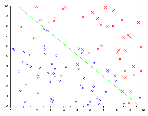
Looks good.
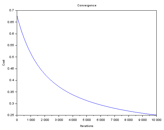
Convergence of the model
The graph of the cost at each iteration is:
// Plot the convergence graph

clf(2);scf(2);
plot(1:n_iter, J');
xtitle('Convergence','Iterations','Cost')
Credits/licence:
Article kindly contributed by Vlad Gladkikh (Copyright owner)
Layout by Yann Debray @ Scilab
More resources:
MOOC on Cousera about Machine Learning from Andrew Ng, Stanford University
https://www.coursera.org/learn/machine-learning/home/welcom