Wind Speed Analysis

This tutorial was kindly contributed by Heinz Nabielek.

1. Measured wind speed data

 

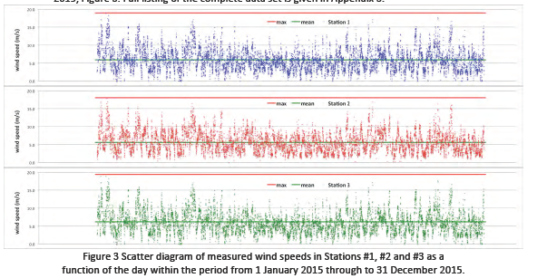
Figure 1 Time series display of 10-minute measured hub-level wind speeds at three
neighbouring stations in the period 1 January 2015 through to 31 December 2015.

// Read measured data //

v=[];

[fd, SST, Sheetnames, Sheetpos] = xls_open('1.xls');

[Value, TextInd] = xls_read(fd, Sheetpos(1));

v=[v Value];

[fd, SST, Sheetnames, Sheetpos] = xls_open('2.xls');

[Value, TextInd] = xls_read(fd, Sheetpos(1));

v=[v; Value];

[fd, SST, Sheetnames, Sheetpos] = xls_open('3.xls');

[Value, TextInd] = xls_read(fd, Sheetpos(1));

v=[v; Value];

clear SST Sheetnames Sheetpos TextInd Value ans fd

mean(v) // mean wind speed in m/s from all 155,808 measurements

ans  =    6.1762483
 

2. Display all measured data as cumulative distribution

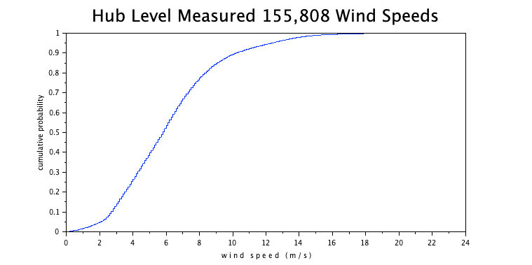
Figure 2 The cumulative probability of the measurement values is a regular function of wind speeds .

 

n=length(v)

vv=gsort(v,'g','i');

yv=(1:n)'/(n+1);

plot(vv,yv);

xtitle('Hub Level Measured 155,808 Wind Speeds',
'w i n d   s p e e d   ( m / s )',
'cumulative probability');
title('Hub Level Measured 155,808 Wind Speeds','fontsize',5);

3. Least-squares fit of measured data with a Weibull distribution

The cumulative wind speed distribution can be approximated by a 2-parameter Weibull distribution W = 1 - exp[ -(v/v_c)^m] , where v_c is the characteristic speed and m is the Weibull modulus, a shape parameter. We can transform this into a linear correlation

m·ln v - m·ln v_c = ln [- ln(1-W)]

and obtain v_c=6.93 m/s and m=2.15 from the least-squares fitting process. However, with wind turbine cut-in speeds of 3 m/s, we selected only wind speeds ³ 3 m/s in the fitting process.

 

low=find(vv>2.99,1);ly=log(-log(1-yv(low:n)));lx=log(vv(low:n));

M=[ones(low:n)' lx];

a=M\ly; m=a(2), vc=exp(-a(1)/m), vm=vc*gamma(1+1/m)

m= 2.1539393  vc= 6.9291892   vm= 6.1365326

plot(vv,yv);xxx=linspace(0.5,22.5,44);plot(xxx, 1-exp(-(xxx/vc)^m),'ro');

xtitle('Distribution of Wind Speeds',
'w i n d   s p e e d   ( m / s )','cumulative probability');

title('Distribution of Wind Speeds','fontsize',5);

legend('155,808 wind speed measurements',
'least-squares fit of a 2-parameter Weibull curve',4);

The derived mean wind speed 6.14 is a bit different from the earlier 6.18 m/s as a result of the selected fit.

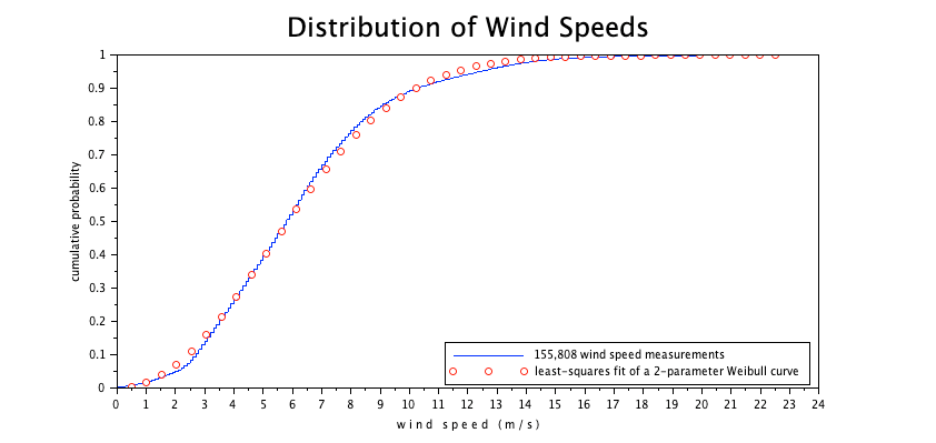
Figure 3 Measured wind speed and fit of a Weibull curve with v_c= 6.93 m/s and m= 2.15  .

Both the measured distribution as also the fitted distribution can be used to predict effective power generation by multiplication with the turbine specific performance curve:

• Zero power until cut-in speed 3 m/s.
• Increase of performance with the 3. power of wind speeds up to 10.7 m/s
• Full power up to 25 m/s, afterwards shutdown for safety reasons.

With the available data, we compute a ~28% capacity factor or equivalent number of full-load-hours.

 

function [y]=eff(x)

y=min(((x/10.7).^3),1) .* (x>3) .*(x<=25)

endfunction

xx=0:.1:31;EFF=eff(xx);

vc=histc(-0.05:.1:31.05,v);

ee=vc*EFF'

ee= 0.275903

scf(4);histplot(-0.5:30.5,v,style=2);plot2d2(xx,EFF/10,style=5);

drawaxis(x=30,y=0:0.02:0.10,dir='r',tics='v',val=string(0:20:100)+' %');

xtitle('Wind speed distribution and Turbine performance yield a 27.6% capacity factor','w i n d    s p e e d   ( m / s )','probability or relative performance');

legend('measured wind speed data', 'typical turbine performance');

 

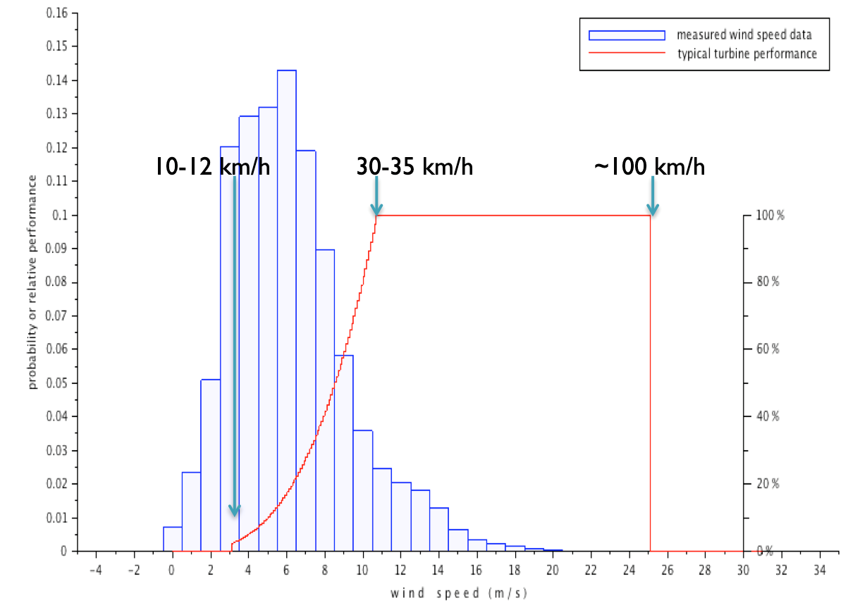
Figure 4 The product of wind speed frequencies with the turbine performance curve can be used for the prediction of the station's capacity factor, here ~28%. It is unfortunate that wind speeds and top turbine performance have only a limited overlap.

 

 

For the case that detailled wind speed measurements are not available, the International Standard IEC61400-12-1 recommends to use the one-parameter Rayleigh distribution W_R= 1 - exp[ -(v/v_c)²] , where v_c is the characteristic speed to be obtained from mean wind speed v_m via v_c~=1.13 v_m. In more detail:

 

 

function [y]=eff(x)

y=min(((x/10.7).^3),1) .* (x>3) .*(x<=25)

endfunction

xx=0:.1:31;nn=length(xx);

xxx=xx(1:(nn-1))+0.05;EFF=eff(xxx);

 

m=2;

M=[];

for vm=3:11; // mean wind speeds of prospective wind farms

vc=vm/gamma(1+1/m); //characteristic wind speed

W= 1 - exp(-((xx+0.05)/vc)^m); w=W(2:311)-W(1:310);

M=[M; vm w*EFF'];

end;

M  =

   3.    0.0367008

   4.    0.0934479

   5.    0.1765748

   6.    0.2732773

   7.    0.3692847

   8.    0.4560266

   9.    0.5296056

   10.   0.5883883

   11.   0.6319652

 

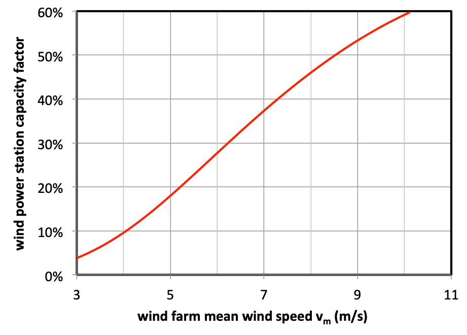
Figure 5  The capacity factor of wind power stations are determined by the wind speed distribution. Here we use the IEC recommended Rayleigh distribution that is equivalent to a Weibull with m=2.

 

4. Simulated wind speeds using Weibull deviates 

Given the cumulative distribution W=W(v), we can generate random deviates via v_random=W^-1(U) where U are [0, 1] uniform random deviates. In our case of Weibull, we perform the transformation

v_random = v_c (- ln U)^1/m,

where v_c is the characteristic velocity and m Weibull modulus. However, it can be quickly seen that these Monte-Carlo simulated time series has no resemblance to measured wind speed time series, Figure 6 .

n=31*24*6  //number of time steps in January 2015
n =    4464.

subplot(2,1,1), plot(v(1:n)),
ylabel('w i n d   s p e e d   ( m / s )');xtitle('a) Measured Wind Speed');

subplot(2,1,2),
plot(vc*((-log(grand(1,n,"def")))^(1/m)),'mo','markersize',0.02);
ylabel('w i n d   s p e e d   ( m / s )');
xtitle('b) Weibull random wind speeds');

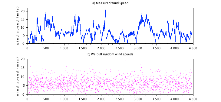
Figure 6  Ten-minute-interval wind speed measurements (a) and random simulation (b) with same frequency distribution over one month, January 2015, measured at hub level. 

The reason for the discrepancy between measurement and simulation is clearly due to the fact that wind speeds are not completely random (not i.i.d.  = independent identically distributed): when the wind blows, it will keep blowing for a little while.....

 

Autocorrelation analysis is the mathematical tool to analyse this situation, here for all 155,808 wind speed data:

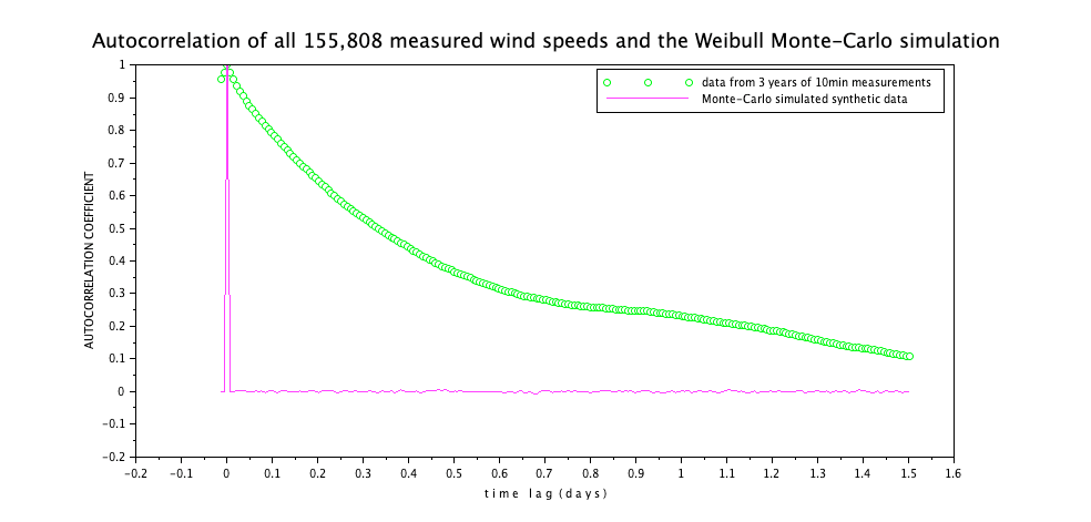
Figure 7 Finite 1.5-day-autocorrelation of measured wind speeds. Beyond 1.5 days do measured wind speeds show no autocorrelation. Weibull deviates simulating wind speeds demonstrate a complete lack of autocorrelation.

[c ind]=xcov(v,"coeff");

l=(length(ind)+1)/2

l= 155808.

plot(ind(l-2:l+216)'/144,c(l-2:l+216),'go');

ll=length(v)

ll= 155808.

w=vc*((-log(grand(1,ll,"def")))^(1/m));

[c ind]=xcov(w,"coeff");plot(ind(l-2:l+216)/144,c(l-2:l+216),'m-');

xtitle('Autocorrelation of all 155,808 measured wind speeds and the stochastic speed simulation',
't i m e   l a g  ( d a y s )','AUTOCORRELATION COEFFICIENT');

title('Autocorrelation of all 155,808 measured wind speeds and the Weibull Monte-Carlo simulation','fontsize',4);

legend('data from 3 years of 10min measurements',
'Monte-Carlo simulated synthetic data');