Computer Vision – Perspective
This tutorial was kindly contributed by Tan Chin Luh, Tritytech.
It leverages the Scilab Computer Vision Module:
https://atoms.scilab.org/toolboxes/scicv/
Perspective transform is slightly more complicated than Affine Transform, where the transformation matrix is a 3×3 matrix to transform image from 3d view into 2d image.
It is quite hard to manually construct the transformation matrix as what we have done in Affine transform, however, it could be easily done with the help of Scilab with linear algebra, or even easier with Scilab SCICV module.
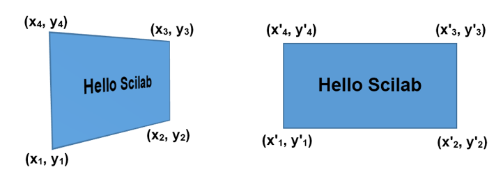
This tutorial will show you how to obtain the transformation matrix from 2 sets of 4 points from the image, where the first set of points indicates the source while the second set for the target.
Transformation Matrix
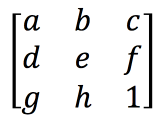
Transformation matrix is the matrix which describe how image pixels remap to a new location to form a transformed image. The transformation matrix for perspective transform is given in the following form:
Finding Transformation Matrix from The Source and Target Points
Function below perform some simple linear algebra operations to find the transformation matrix from the sets of source and target points. (4 points each).
// Tentative workaround for getPerspectiveTransform

function mat=getPerspectiveTransform2(src, tgt)
    src1 = [src(:,1:3); 1 1 1];
    src2 = [src(:,4);1];
    tgt1 = [tgt(:,1:3); 1 1 1];
    tgt2 = [tgt(:,4);1];
    a = src1\src2;
    b = tgt1\tgt2;
    A = src1.*repmat(a,1,3)';
    B = tgt1.*repmat(b,1,3)';
    mat = B*inv(A);
endfunction
This is the current workaround for the SCICV in which the PtList does not support insertion yet, and once the coming release support this, it could be simply replaced with the build in function. For now, bear with me by using this function.
Perspective Transformation
The codes below is an interactive program, just run these lines with the above function (getPerspectiveTransform2) loaded, you would be prompt to select 4 points for source and target separately, and you would see the transformed image at the end of the program.
If you’re still unsure what to do, view this 26-second video first:
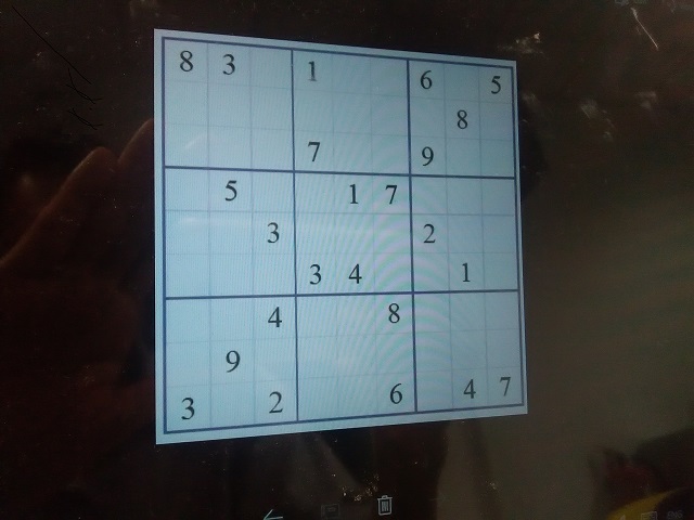
// Import image
scicv_Init();
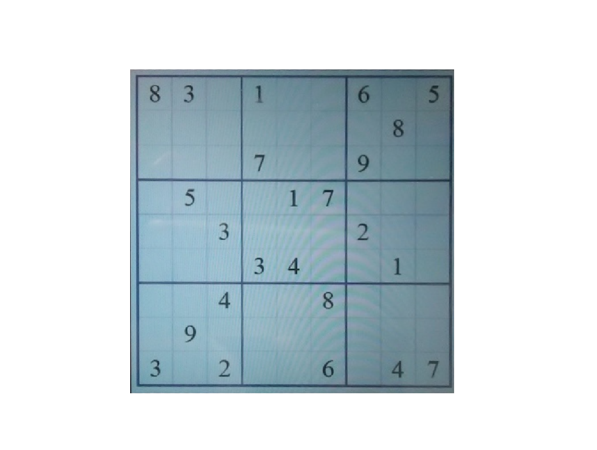
S=imread('sudoku1.jpg');
// Select 4 points from the figure (interactive)
matplot(S);
set(gca(), "mark_foreground",5);
messagebox('Now select 4 corners of the puzzle','Select Points','modal');
src = locate(4,1);
messagebox('Source Points selected','Done','modal');
messagebox('Now select another 4 points on the image, preferable a square','Select Points','modal');
tgt = locate(4,1);
messagebox('Target Points selected','Done','modal');
sz = size(S)
src(2,:) = sz(1) - src(2,:);
tgt(2,:) = sz(1) - tgt(2,:);
mat = getPerspectiveTransform2(src,tgt)
// Find the transformation matrix and perform the transformation
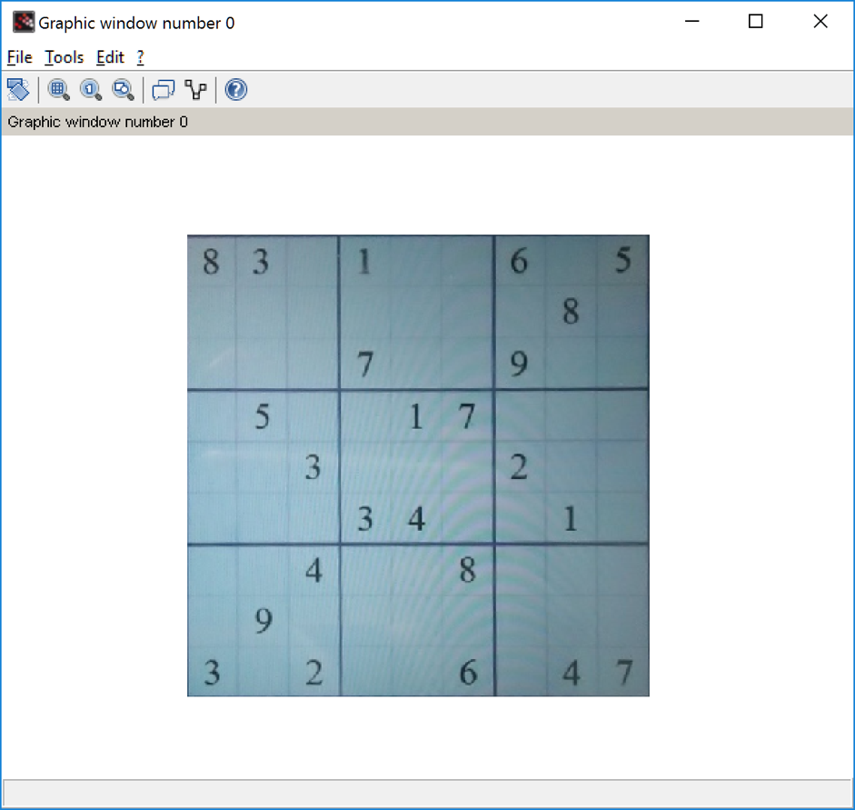
Snew = warpPerspective(S,mat,size(S));
matplot(Snew);
You could also manually select your own target points to have a better projection. For example, mapping to the target of 480×480 pixels image could be done by:
// Manually select target points
tgt = [0 0;0 sz(1);sz(1) sz(1);sz(1) 0]';
mat = getPerspectiveTransform2(src,tgt)
Snew = warpPerspective(S,mat,size(S));
Snew2 = Snew(1:sz(1),1:sz(1));
matplot(Snew2);
Detecting the Source Points with HoughLine Transform
In order to detect the source points automatically, a few transformations are available to detect the lines of the square, and then we could use linear algebra method to find the intersection points to form our source points.
In this example, we are going to use the HoughLine Transform for this purpose.
First of all, we need to pre-process the image in order to get the borders of the big square:
// Import image
scicv_Init();
S=imread('sudoku1.jpg');

// Process image to find the box
S_gray = cvtColor(S,CV_RGB2GRAY);
sz = size(S_gray);
[thresh, S_bin] = threshold(S_gray, 0, 255, THRESH_OTSU);

// Morphology to close the holes, left the big square box for the sudoku puzzle
se = getStructuringElement(MORPH_RECT, [7 7]);
S_close = morphologyEx(S_bin, MORPH_CLOSE, se);

// Edge detection to find the lines of the big square
E = Canny(S_close, 0, 1, 5);

subplot(221); matplot(S); title('Original Image');
subplot(222); matplot(S_bin);title('Binary Image');
subplot(223); matplot(S_close);title('Closing Image');
subplot(224); matplot(E);title('Edge Image');
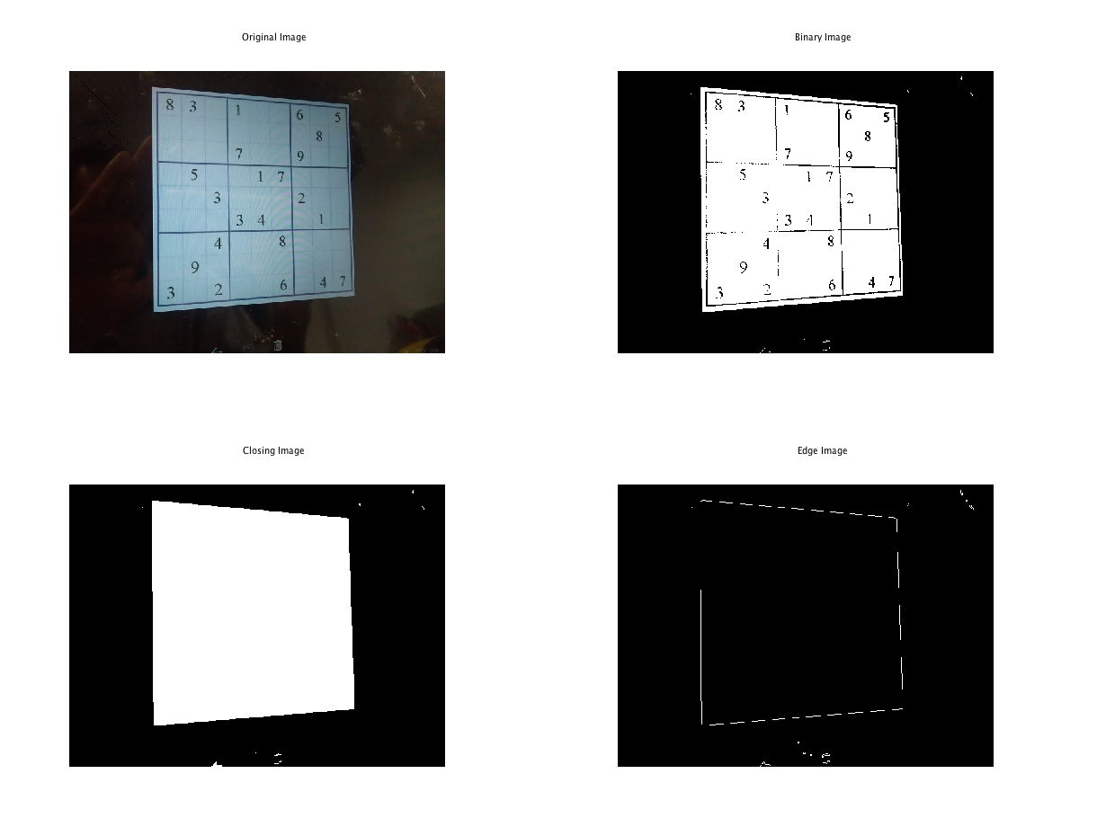
With the binary image with clean edge of the square, we could use the HoughLine transform of find the straight-line parameters, and then the intersection points:
// Detect straight lines using HoughLine Trasnform
L = HoughLines( E, 1, CV_PI/180,100);
// Creating 4 lines
rho = L(:)(:,2);
theta = L(:)(:,1);
aa = cos(theta);
bb = -sin(theta);
x0 = aa.*rho, y0 = bb.*rho;
pt1 = [round(x0 + 500*(-bb)),round(sz(1) + y0 + 500*(aa))];
pt2 = [round(x0 - 500*(-bb)),round(sz(1) + y0 - 500*(aa))];
scf();
matplot(S_gray);
gca().auto_scale = 'off';
for cnt = 1:size(pt1,1)
plot([pt1(cnt,1),pt2(cnt,1)],[pt1(cnt,2),pt2(cnt,2)],'r');
end
// find horizontal lines and vertical lines
theta_deg = theta.*180/%pi;
hline = (theta_deg > -45 & theta_deg 135 & theta_deg
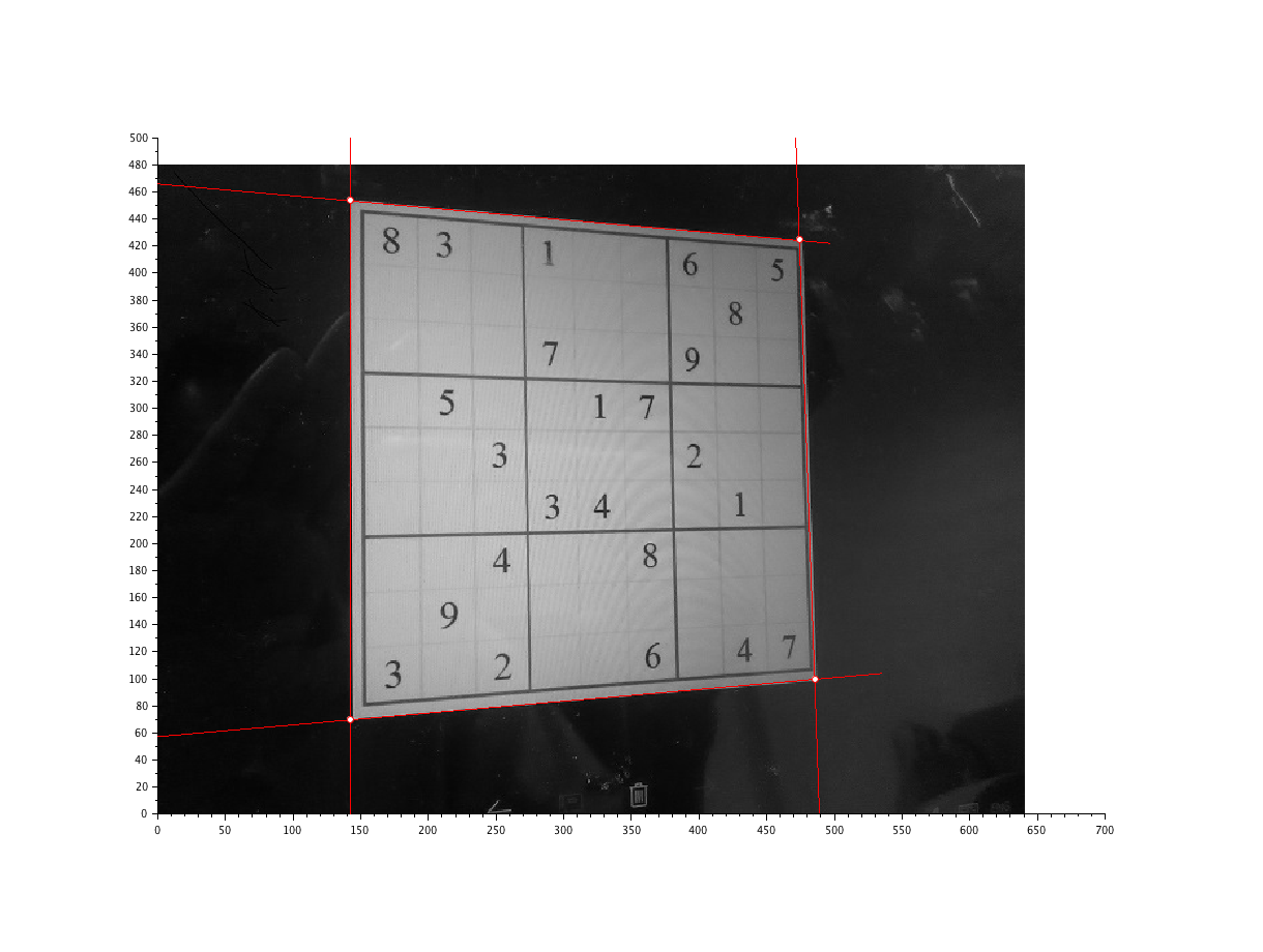
Finally, we transform the image with the points found.
// Convert from cartesian coor to image coor
XY_int = pts';
XY_int(:,2) = sz(1) - XY_int(:,2);
// Perform Perspective Transform and remap the image to new coordiates
src = gsort(XY_int,'lr','i');
tgt = [0 0;0 sz(1);sz(1) 0;sz(1) sz(1)];
mat = getPerspectiveTransform2(src',tgt');
// Find the transformation matrix and perform the transformation
Snew = warpPerspective(S,mat,size(S));
//matplot(Snew);
Snew2 = Snew(1:480,1:480);
scf();
matplot(Snew);
Similar code with Scilab IPCV toolbox could be found at the link below.
Coming up: Solve the Sudoku puzzle!