Computer Vision – Image2Data

This tutorial was kindly contributed by Tan Chin Luh, Tritytech.

It leverages the Scilab Computer Vision Module:
https://atoms.scilab.org/toolboxes/scicv/

The code below requires the “imselect” function extracted from IPCV module.

Scilab could be used together with its Image Processing module to extract points from a line in an image, either manually or automatically.

This tutorial will show you a simple manual way to extract the points by using mouse clicks, and then trying to fit the points to make a better guess for a sine wave.

Image with Line(s)

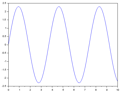
The image shown below is generated by Scilab for this tutorial, you could either save the image to work directly or generate your own image with the following lines:

 

// Generating your own line

x = 0:0.1:10;

y = 2.3*sin(2*%pi*1.7);

plot(x,y);

 

This is followed by choosing the “Export To” menu item and save it as an image, for this tutorial, it assumes that we have saved the image with the name of “ex1.png”.

 

Reading Image and Selecting Data Ragne.

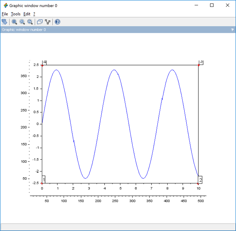
We have to know the data bounds from the image, so first of all, we load the image and let the user choose the four corners points as shown in the figure below.

 

// Read the Image and select range

scicv_Init();

S = imread('ex1.png');

matplot(S);replot('tight');

pts = imselect(4)

x_min = min(pts(:,1));

x_max = max(pts(:,1));

y_min = min(pts(:,2));

y_max = max(pts(:,2));

 

The function “imselect” (see appendix) is used to perform this, and for this case, we let the function knows that we are going to choose only 4 points. The points are then used to compute the boundary information for the data and saved into 4 variables namely x_min, x_max, y_min and y_max.

 

Choosing Data Points

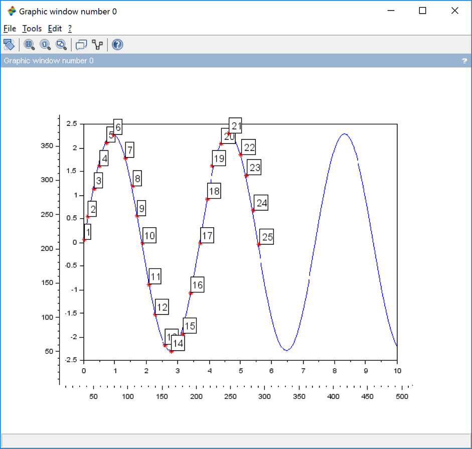
Now we let the user to choose the data points on the image. Do note that even though the “imselect” is giving 100 as parameter, meaning that the user could choose up to 100 points, however, we could always end the selection by using right mouse button click.   

// Choose Data Points

matplot(S);replot('tight');

pts2 = imselect(100);

x_img = pts2(:,1);

y_img = pts2(:,2);

 

Represent the selected Data Points

With boundary information and the data selected by the user, we now compute the estimated x and y.

// Normalized Data to convert data into range of [0 1]

x_norm = (x_img - x_min)/(x_max - x_min);

y_norm = (y_img - y_min)/(y_max - y_min);

// "Denormalized" using the boundary to convert data into the range given.

x_min_actual = 0;

x_max_actual = 10;

y_min_actual=-2.5;

y_max_actual=2.5;

x_est= (x_norm*(x_max_actual - x_min_actual) + x_min_actual)

y_est =(y_norm*(y_max_actual - y_min_actual) + y_min_actual)

plot(x_est,y_est);

 

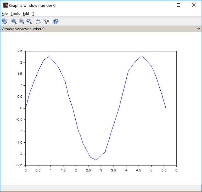
Make It Better By Fitting The Data

As we could see from the previous image, the graph is not smooth due to the selected points are limited. Let’s try to estimate the sine wave parameters and find the equation of the line so that we could get a nice plot.

// Fitting the data with least square method

function y=my_func(x, p)

   y  = p(1)*sin(p(2)*x)

endfunction

function e=err_func(p, xm, ym, wm)

   e = wm.*( my_func(xm, p) - ym )

endfunction

wm = ones(x_est);

p0 = [3 ; (2*%pi)/4]; // Guess from the image

[f,p_predict, g] = leastsq(list(err_func,x_est,y_est,wm),p0)

x_predict = 0:0.1:10;

y_predict = p_predict(1).*sin(p_predict(2).*x_predict);

plot(x_est,y_est,'b.-');

plot(x_predict,y_predict,'r');

 

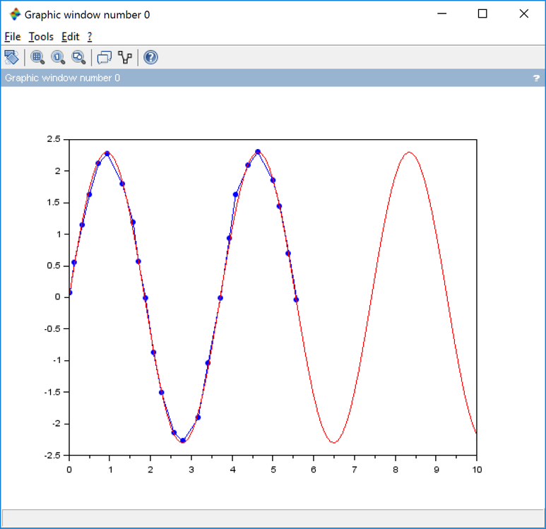
--> p_predict 
p_predict  =     

2.3005639   
1.6950462