Computer Vision – Image Transform
This tutorial was kindly contributed by Tan Chin Luh, Tritytech.
It leverages the Scilab Computer Vision Module:
https://atoms.scilab.org/toolboxes/scicv/
Affine Transform usually are used for translation, rotation and scaling of an image to correct its alignment which is distorted or deformed due to the imperfection of hardware (camera), or human error while snapping the image.
This tutorial will show you how to use Affine transform features in Scilab Computer Vision module to perform following operations:
- Translation
- Rotation
- Scaling
- Shearing
Transformation Matrix
Transformation matrix is the matrix which describe how image pixels remap to a new location to form a transformed image. The following table summarizes the affine transform matrices for the operations mentioned above.
| Operation | Transformation Matrix |
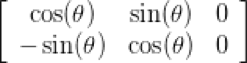
| Translation | |
| Rotation | |
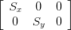
| Scaling | |
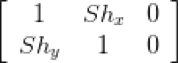
| Shearing |
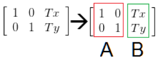
Matrix Operation of Transformation Matrix and The Image Pixels.
Let’s look into the fundamental on how the transformation matrix is used to transform the image. We will use the translation matrix for this example.
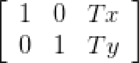
Transformation Matrix:
Let [x;y] be an coordinate (location) of a pixel, say, [1;1]:
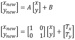
In Scilab code;
--> new_loc = [1 0;0 1]*[1;1] + [2;2]
new_loc =
3.
3.
This means the pixel value located in location [1;1] would be reallocated to new location [3;3].
Affine Transformation
Following codes using SCICV module for the Affine Transform for translation, rotation, scaling and shearing.
scicv_Init();
S = imread(getSampleImage("lena.jpg"));
matplot(S);
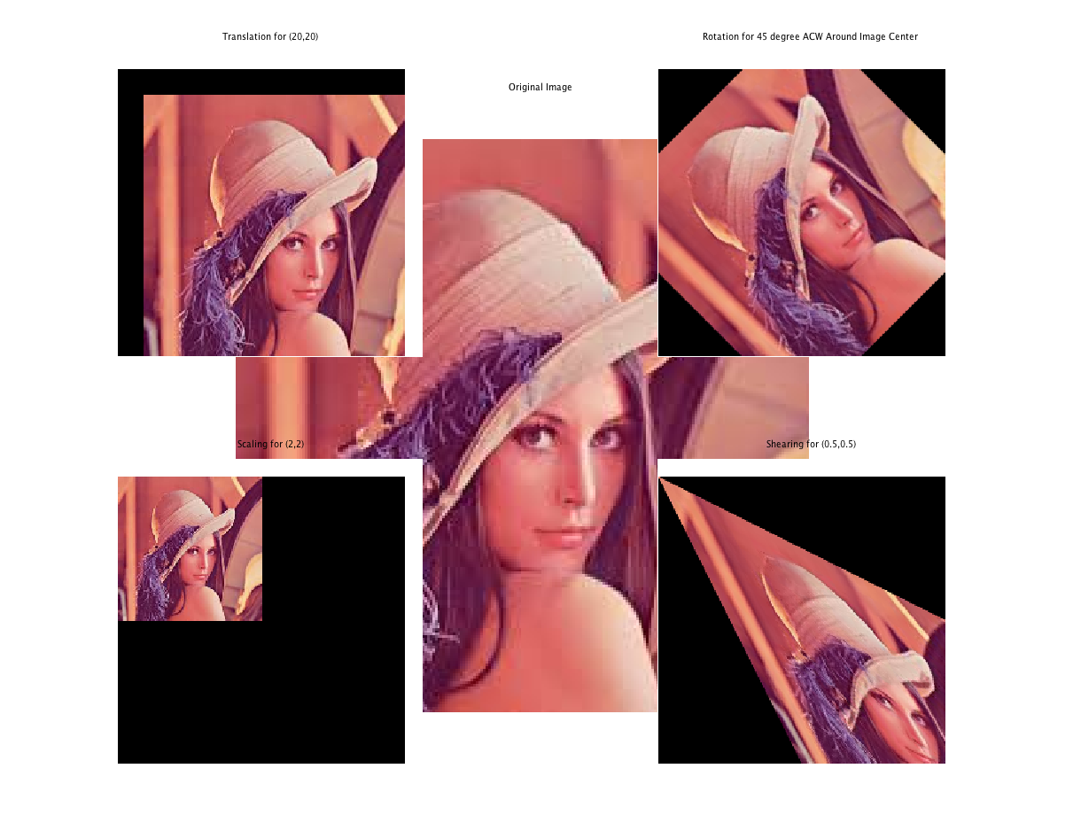
title('Original Image');
//////////////////////////
// Translation for (20,20)
//////////////////////////
mat = [ 1 0 20;...
0 1 20];
S2 = warpAffine(S, mat, size(S));
subplot(2,2,1);
matplot(S2);
title('Translation for (20,20)');
//////////////////////////
// Rotation for theta = 45 degree Arond Image Center
//////////////////////////
sz = size(S);
theta = 45*%pi/180;
Alpha = sin(theta);
Beta = cos(theta);
// The rotational operation would performed around image origin (0,0),
// if we were to rotate around the center of image,
// we need to translate the image with the following formulas
Tx = (1-Beta)*sz(2)/2-Alpha*sz(1)/2;
Ty = Alpha*sz(2)/2+(1-Beta)*sz(1)/2;
mat = [ Beta Alpha Tx;...
-Alpha Beta Ty];...
S3 = warpAffine(S, mat, size(S));
subplot(2,2,2);
matplot(S3);
title('Rotation for 45 degree ACW Around Image Center');
//////////////////////////
// Scaling Factor of 0.5
//////////////////////////
mat = [ 0.5 0 0;...
0 0.5 0];...
S4 = warpAffine(S, mat, size(S));
subplot(2,2,3);
matplot(S4);
title('Scaling for (2,2)');
//////////////////////////
// Shearing for (0.5,0.5)
//////////////////////////
mat = [ 1 0.5 0;...
0.5 1 0];...
S5 = warpAffine(S, mat, size(S));
subplot(2,2,4);
matplot(S5);
title('Shearing for (0.5,0.5)');
delete_Mat(S);
delete_Mat(S2);
delete_Mat(S3);
delete_Mat(S4);
delete_Mat(S5);
Note: I purposely overlap the original image behind the 4 transformed images. If you find this annoying, simply add a line to show them on different figure.
As a conclusion, you can observe this animation explaining all 4 transformations:
![]()
Go here to view the code:
http://scilabipcv.tritytech.com/2017/07/04/understanding-transformation…