System parameter identification
This tutorial displays a typical use case of optimization of control systems. The identification of parameters for a controller usually proceeds in the following steps:
- Data acquisition of the system to regulate in open loop
- Modeling the dynamic system
- Identification of the system parameters
- Set up of a control strategy (simple PID, to more evolve Model Predictive Control)
Example :
Second order system

Running a simulation with a unit step input (with the parameters K, Tau et Tau2 all equals 1):
Introduction of the block “to workspace” to gather the results of the simulation in the Scilab environment for post-processing:
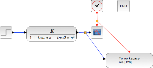
Those results are then accessible through the variable res, contening 2 fields :
- values
- time
Next step: Write an optimization script running Xcos in batch to identify the 3 parameters of the second order system (K, Tau and Tau2).
Defining a cost function returning y, the distance between the simulated curve of the system and the unit step input function.
function y=cost_for_fminsearch(x)
    context = ["K="+string(x(1)) "tau="+string(x(2)) "tau2="+string(x(3))];

    // On impose un cout infini si on sort de nos bornes de recherche.
    if x(1) < 0 | x(2) < 0 | x(3) < 0 then
        y=%inf
        return
    end

    try
        // Ouverture du diagramme => cree une variable scs_m
        importXcosDiagram(pwd()+"/Asserv_2nd_ordre.zcos");
        // Changement du contexte
        scs_m.props.context = context;
        // Simulation
        xcos_simulate(scs_m, 4);
    catch
        disp("Error during xcos Simulation ...");
        error("cost function failed.")
        y = %inf;
        return
    end

    res_ref = ones(40,1);
    y = norm(res.values - res_ref)^2;
    e = get("costPolyline");

    e.data(:, 2) = res.values;
endfunction
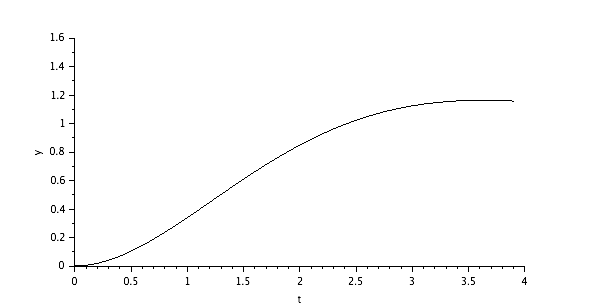
The results are represented dynamically from this script iterating until finding the optimal solution in the defined interval:
f = gcf();
plot([0, 3.9], [1, 1], "r");
plot([0:0.1:3.9], zeros(40, 1));
e = gce();
e.children(1).tag = "costPolyline";
a = gca();
a.data_bounds = [0, 0 ; 4, 1.8]
The optimization function called to identify the 3 systems parameters is fminsearch :
opt = optimset( "Display" , "iter" );
[x fval] = fminsearch ( cost_for_fminsearch , [0 0 0] , opt );
The calling syntax of this function is:
- Cost function defining the quantity to minimize:
cost_for_fminsearch - Starting point of the search:
[0 0 0] - Advanced options with the function optimset:
options.Display = "iter" → the algorithm returns a message at each iteration
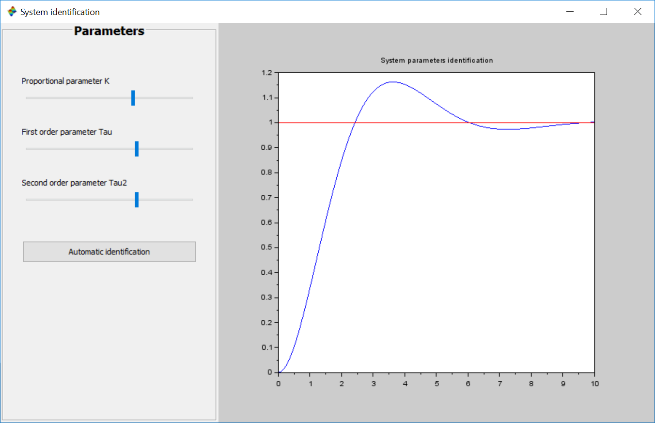
You can develop a Graphical User Interface (GUI) to modify manually the 3 parameters or trigger the automatic identification. Read the following tutorial to find out how.

This work is licensed under a Creative Commons Attribution-ShareAlike 4.0 International License.