System elements modeling – the inertial element
This article was originally published on x-engineer.org
Thanks to x-engineers for their contribution.
—
The behavior of some mechanical systems is identical to that of certain electrical systems. Therefore, we can have an unified modeling approach when dealing with mechanical and electrical system modeling.
Mechanical and electrical lumped parameters systems can be modeled with basic elements. These elements are: the inertial element, the compliant element and the resistive element.
As the name suggests, the inertial element is contained in systems with inertia. Mechanical, electrical, hydrodynamic and thermal systems have inertia. The property of inertia is to resist change of current state (e.g. velocity).
Mechanical systems
Image: Translation of a rigid body
An example of inertial element is a moving (translational or rotational) body. If a force F is applied to a rigid body with mass m, it will start to move with a velocity v.
The force applied to the mass is equal with the derivative of the translational momentum pt.
F=dpt /dt
The translational momentum is the product between the mass m and the velocity v.
pt=m⋅v
With x being the position of the body, v the velocity and a the acceleration, we can write the mathematical relation of the force F and mass m.
F=m.d²x/dt²=m.dv/dt=m.a
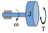
Image: Rotation of a rigid body
The same approach can be applied to a rotational rigid body with a moment of inertia J. If we apply a torque T to the body, it will start to rotate with the angular velocity ω.
The torque applied to the moment of inertia is equal with the derivative of the rotational momentum pr.
T=dpr/dt
The rotational momentum is the product between the moment of inertia J and the angular velocity ω.
pr=J⋅ω
With α being the angular position of the body, ω the angular velocity and ε the angular acceleration, we can write the mathematical relation of the torque T and moment of inertia J.
T=J.d²α/dt²=J.dω/dt=Jϵ
Electrical systems
Looking into electrical systems we can also identify the inertial element.
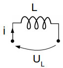
Image: Inductor electrical symbol
An electrical circuit with an inductor is characterized by an inductance L, a current i and a voltage drop across the inductor UL.
The equivalent electrical parameter for the momentum is the flux linkage λ.
λ=L⋅i
The voltage drop on the inductor is equal to the derivative of the flux linkage.
UL=dλ/dt
In the electrical domain the inertial element is the inductance. With q being the charge, i the electric current and di/dt the variation in time of the electric current, we can write the mathematical relation of the voltage drop UL and inductance L.
UL =L.d²q/dt²=Ldi/dt
We can now write an equivalency table between the mechanical (translational and rotational) and electrical system for the inertial element.
| Mechanical | Electrical | |
| Translational | Rotational | |
| Force, F | Torque, T | Voltage, UL |
| Linear acceleration, a | Angular acceleration, ε | Current variation, di/dt |
| Linear velocity, v | Angular velocity, ω | Electrical current, i |
| Linear position, x | Angular position, α | Electrical charge, q |
| Mass, m | Moment of inertia, J | Inductance, L |
If we look at the relationships of force (1), torque (2) and voltage (3), we can see that the inertia acts as a slope of the linear dependencies.
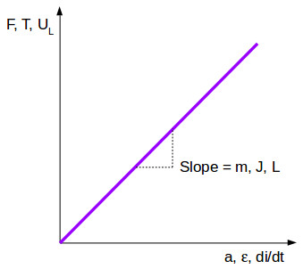
Image: The law of inertia
For a better understanding of the behavior of the inertial element in a dynamic system, we are going to use a Xcos block diagram in which we integrate the differential equation of the translational body (1).
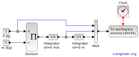
Image: Xcos model – inertial element with constant force
In this example we consider the force as being constant. The initial conditions of the position and velocity are 0. The simulation results are stored in a structured variable simOut.
By using a post-processing Scilab script, we plot the force, speed and position for the translational rigid body.
clc()
subplot(3,1,3)
plot(simOut.time,simOut.values(:,1)), xgrid()
ylabel('F [N]')
xlabel('t [s]')
subplot(3,1,2)
plot(simOut.time,simOut.values(:,2)), xgrid()
ylabel('v [m/s]')
subplot(3,1,1)
plot(simOut.time,simOut.values(:,3)), xgrid()
ylabel('x [m]')
Running the Scilab script will output the following graphical window:
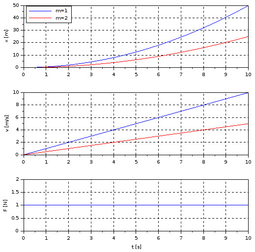
Image: The velocity and position of the inertial element for constant force
By analyzing the above plot we can notice that the velocity accumulates over time, it does not have sudden value changes. Also the higher the mass, the higher the inertia, the “harder” to change the position of the rigid body, for the same input force.
Now we’ll analyze the impact of a sudden force change on the behavior of the system. For this we use the same Xcos model, the only difference being the input force, which will change in time.
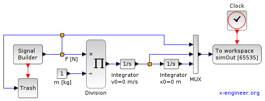
Image: Xcos model – inertial element with variable force
Running the Xcos model and the post-processing Scilab script gives the following graphical window:
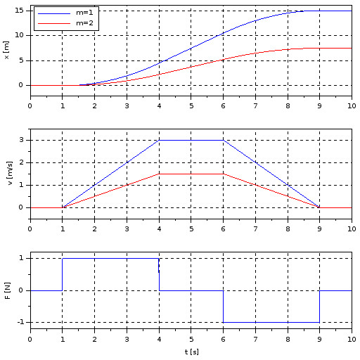
Image: The velocity and position of the inertial element for variable force
When there is a “step” change of the input force, the velocity changes continuously, without steep variations. When the input force is 0, the acceleration is 0, the velocity is constant and the position changes after a linear law (between seconds 4 and 6).
In a dynamic system with inertia, we can not impose steep variations of the speed or electrical current. Their value changes over time, depending of the value of the input force or voltage.
Remember that any dynamic system with mass, moment of inertia or inductance has inertia.
For any questions, observations and queries regarding this article, use the comment form below.
Don’t forget to Like, Share and Subscribe!
Read more: