Surface fitting

1. Introduction

Very often, in engineering sciences, data have to be fitted to have a more general view of the problem at hand. These data usually come out from a series of experiments, both physical and virtual, and surface fitting is the only way to get relevant and general information from the system under exam.

Many different expressions are used to identify the activity of building a mathematical surrogate describing the behavior of a physical system from some known data. Someone simply talks about “regression“ or “data fitting” or “data interpolation”, someone else talks about “modeling” or “metamodeling” or “response surface methodology”. Different application fields, and different schools, use different words for describing the same activity.

The common activity is carrying out a mathematical model starting from points. The model should be able to describe the phenomenon and should also give reliable answer when estimating values in unknown points.

This problem is well-known in literature and a wide variety of solutions has been proposed.
In this paper we present a series of techniques which engineers can implement in Scilab and use to solve data fitting problems very easily and fast.
For sake of simplicity, in this tutorial we decided to consider 30 couples of values (x and y, belonging to the interval [0, 1]) to which a system response (z) is associated. The data fitting problem reduces, in this case, to find a mathematical function of kind f(x,y), able to reproduce z at best (see Figure 1).

Of course, all the techniques described hereafter can be extended to tackle
multidimensional data fitting problems.

 

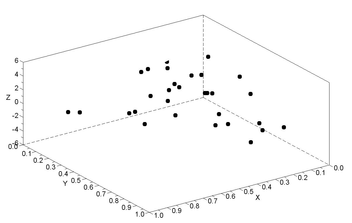
Figure 1: 3D plot of the dataset used in this paper: 30 points.

2. Polynomial fitting

Probably one of the simplest and most used data fitting techniques is the polynomial fitting.
We imagine that the system response can be adequately modeled by a mathematical
function p(x,y) expressed as:

where coefficients represent the free parameters of the model. Usually, polynomial coefficients are determined imposing the interpolation condition of p(x,y) in each point of the dataset (xi,yi) obtaining a system of linear equations, such as:

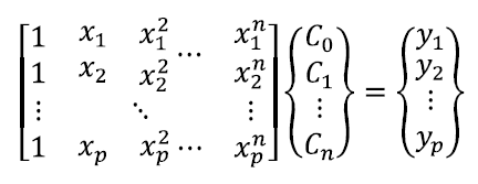
The number of points p to be fitted is usually larger than the number of coefficients of the polynomial. This leads to an over-determined system (more equations than unknowns) which has to be solved in a least square sense. The resulting polynomial generally does not interpolate exactly the data, but it fits the data instead.
It is very easy to set up a Scilab script which implements this fitting technique: the main steps to be performed are to correctly set up the over determined system, whose coefficients can be computed in our case using a Pascal triangle, and the solution of the
system.
The resulting model can be also plotted. In Figure 2 the polynomial of degree 4 is drawn together with the 30 points in the dataset (a.k.a. training points). It can be seen that the surface does not pass through the training points.
One could be tempted to choose a very high degree of the polynomial in order to have a very flexible mathematical model able, in principle, to correctly capture complex behaviors.
Unfortunately, this does not lead to the desired result: the problem is known as “overfitting” or “Runge phenomenon” in honor of the mathematician who described it (see Figure 3).
The risk is that, when increasing too much the polynomial degree, the obtained model
exhibits an oscillatory and unnatural behavior between the dataset points. In other words, the polynomial “over fits” the data, as commonly said in these cases.
This overfitting problem, which is universally known linked to the polynomial fitting, also afflicts other fitting techniques. The “Ockham’s razor” should be kept in mind when dealing with fitting: the suggestion is here to not abuse of the possibility to add complexity to the model when not strictly necessary.

The file polynomial_fitting.sce contains a possible implementation of the polynomial fitting technique described above

 

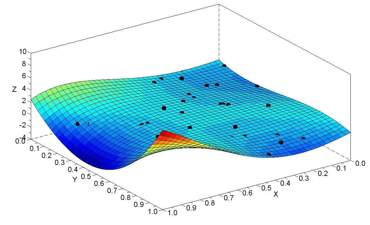
Figure 2: Polynomial of degree 4 is plotted together with the dataset points (black dots). It can be seen that the resulting surface, even if it approximates the data, does not pass through the points, being not interpolating.

 

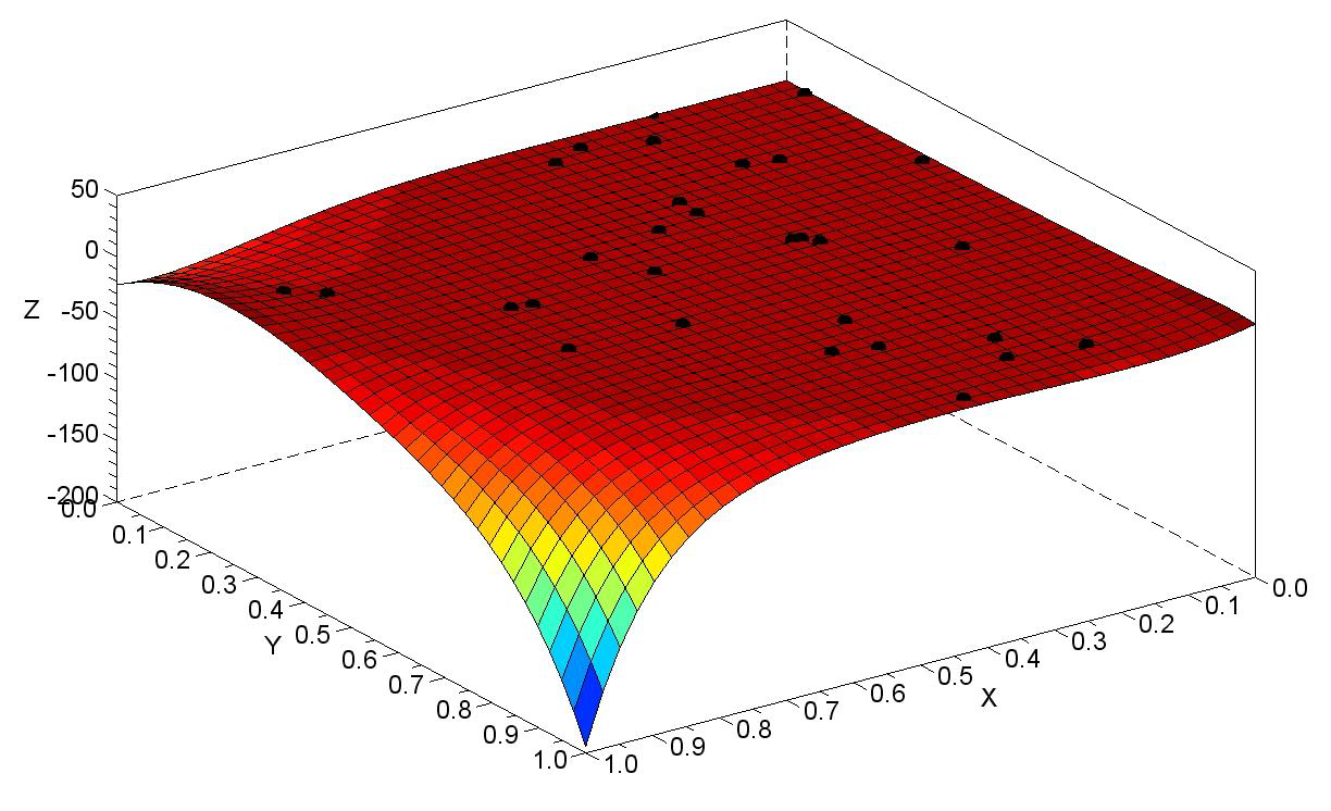
Figure 3: The overfitting phenomenon is plotted in this picture. A 10 degree polynomial is used in this case. The resulting model exhibits large unrealistic oscillations far from the dataset points.