Satellite orbit around the earth

The CNES has been a great user of Scilab, and a long-term partner of us. Upon their advice, we presented one of their use case at the the 6th International Conference on Astrodynamics Tools and Techniques (ICATT).

The question is a classical problem of space mechanics solved step-by-step, to demonstrate the capacities of Scilab in this field:

Download the script (myEarthRotation - PDF)

Download the full tutorial (Scilab Orbite Simulation - PDF)

1.   Express the physics problem

The problem is based on the universal law of gravitation:

 

We write down Newton’s second law of motion in an earth-centred referential:

(1)

 

(2)

 

Position of the satellite is at a distance r [x; y]

Earth mass centre is at O [0; 0]

Gravitational constant:

 

Mass of the earth:

 

Radius of the Earth:

 

2. Translate your problem into Scilab

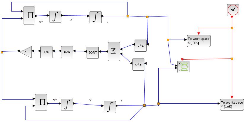
Scilab is a matrix-based language. Instead of expressing the system as set of 4 independent equations (along the x and y axis, for position and speed), we describe it as a single matrix equation, of dimension 4×4:

This method is a classical trick to switch from a second order scalar differential equation to a first order matrix differential equation.

 

with

 

 

To simplify the equation, we define the variable:

 

Open scinotes with edit myEarthRotation.sci

Define the skeleton of the function:

function udot=f(t, u)
    G = 6.67D-11; //Gravitational constant
    M = 5.98D24; //Mass of the Earth
    c = -G * M;
    r_earth = 6.378E6; //radius of the Earth
    r = sqrt(u(1)^2 + u(2)^2);
​
    // Write the relationhsip between udot and u
    if r < r_earth then
        udot = [0 0 0 0]';
    else
        A = [[0     0     1 0];
        [0     0     0 1];
        [c/r^3 0     0 0];
        [0     c/r^3 0 0]];
        udot = A*u;
    end
endfunction
​

The condition defined by the distance r of the satellite with the centre of earth stops the simulation if it’s colliding with earth’s surface.

 

 

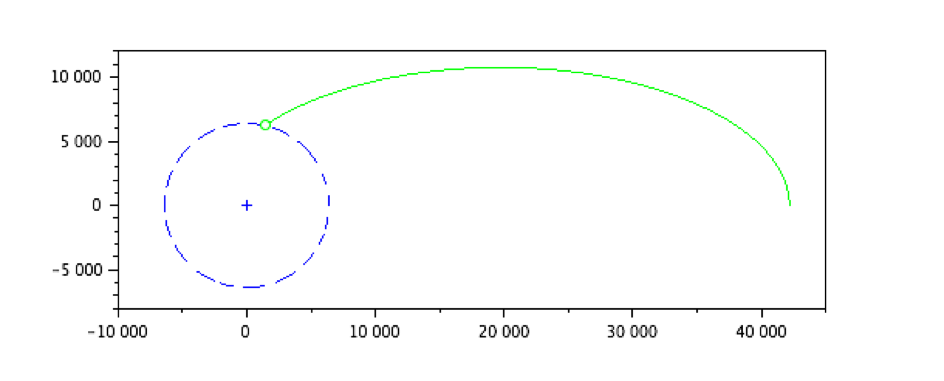
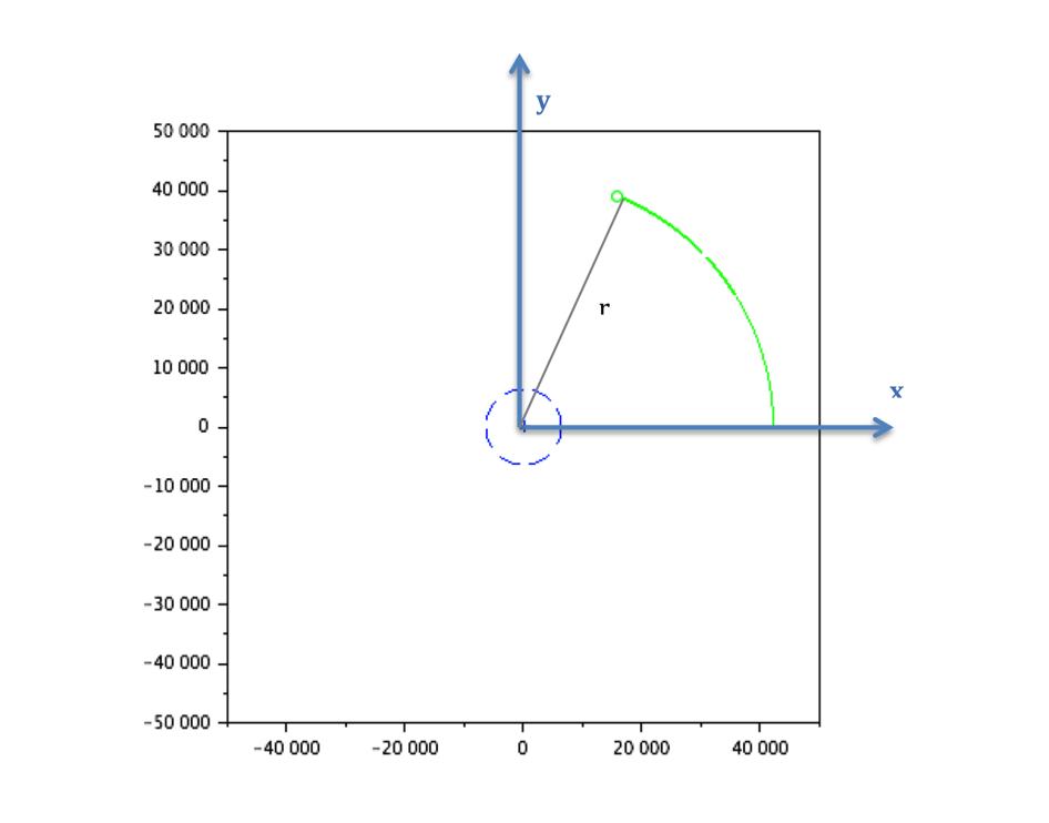
Try out the final script with the following initial conditions in speed and altitude:

--> geo_alt = 35784; // in kms
--> geo_speed = 1074; // in m/s
--> simulation_time = 24; // in hours
--> U = earthrotation(geo_alt, geo_speed, simulation_time);

3.   Compute the results and create a visual animation

With this function, we go to the core of the problem:

function U=earthrotation(altitude, v_init, hours)
    // altitude given in km
    // v_init is a vector [vx; vy] given in m/s
    // hours is the number of hours for the simulation
    r_earth = 6.378E6;
    altitude = altitude * 1000;
    U0 = [r_earth + altitude; 0; 0; v_init];
    t = 0:10:(3600*hours); // simulation time, one point every 10 seconds
    U = ode(U0, 0, t, f);

    // Draw the earth in blue
    angle = 0:0.01:2*%pi;
    x_earth = 6378 * cos(angle);
    y_earth = 6378 * sin(angle);
    fig = scf();
    a = gca();
    a.isoview = "on";
    plot(x_earth, y_earth, 'b--');
    plot(0, 0, 'b+');

    // Draw the trajectory computed
    comet(U(1,:)/1000, U(2,:)/1000, "colors", 3);
endfunction

The resolution of the ordinary differential equation (ODE) is computed with the Scilab function ode.

ode solves Ordinary Different Equations defined by:

 

where y is a real vector or matrix

The simplest call of ode is: y = ode(y0,t0,t,f) where y0 is the vector of initial conditions, t0 is the initial time, t is the vector of times at which the solution y is computed and y is matrix of solution vectors y=[y(t(1)),y(t(2)),…].

Go further

To go further in numerical analysis, find out more about the solvers:

Ordinary Differential Equations with Scilab, WATS Lectures, Université de Saint-Louis, G. Sallet, 2004