Machine Learning – regression tutorial
Regression tutorial
Simple example —
Deducing the value of a house based on the sampled prices of the market
The idea is to find the model which links an important characteristic with the price, and deduce the value of any house.
We choose a polynomial model of order 1 ( y = a*x + b ), which we will fit by linear least squares regression.
This is our sample of the market :
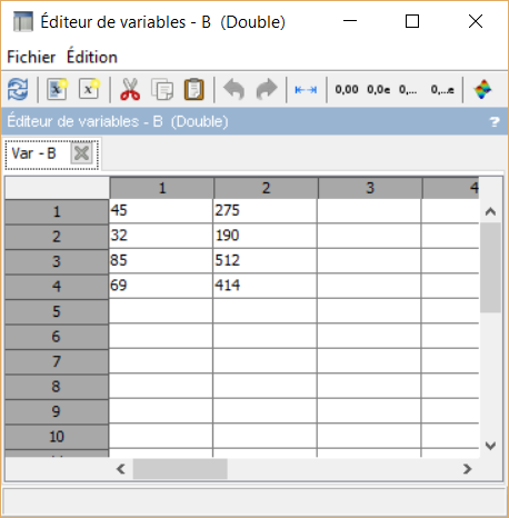
| surface area (m2) | price (Thousand USD) |
|---|---|
| 45 | 275 |
| 32 | 190 |
| 85 | 512 |
| 69 | 414 |
Simply copy and paste the table values in the variable editor:
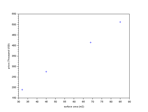
Plot the values as follow:
--> plot(B(:,1),B(:,2),"+")
If there was a perfect polynomial model of order 1 of this market,
we would have the following :
275 = 45 * a + b
190 = 32 * a + b
512 = 85 * a + b
414 = 69 * a + b
What we are looking for are the best a and b — according to a chosen criteria : this is why we talked about least squares. We can grade how good a model is by looking at how far each sample’s estimation is to the actual value.
The distance we choose to calculate is the difference between these values, squared (so that it is always positive and there is only one solution1,2).
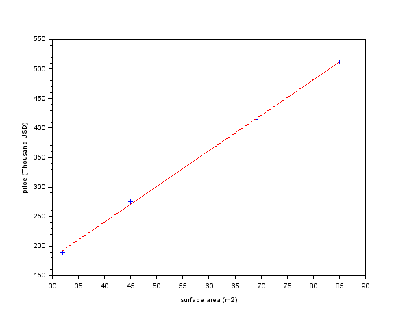
To compute the linear regression of the system, do as follow:
--> x=B(:,1)'
--> y=B(:,2)'
--> [a, b] = reglin(x, y);
--> plot(x, a*x+b, "red"
Next episode: the cost function
For the samples we have given, this is the formula to calculate the
sum of the squared distances (the grade of a model, or cost function) :
S(a, b) = [275 – (a * 45 + b)]2 + [190 – (a * 32 + b)]2 + [512 – (a * 85 + b)]2 + [414 – (a * 69 + b)]2
--> deff("z=S(a,b)",["z = [275 - (a * 45 + b)].^2 + [190 - (a * 32 + b)].^2 + [512 - (a * 85 + b)].^2 + [414 - (a * 69 + b)].^2"])