Machine learning – Neural network function approximation tutorial

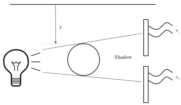
In this tutorial, we will approximate the function describing a smart sensor system. A smart sensor consists in one or more standard sensors, coupled with a neural network, in order to calibrate measurements of a single parameter.

We will consider the voltage v1 and v2 coming from two solar cells, in order to assess the location of an object in one dimension y:

This tutorial is based on the Neural Network Module, available on ATOMS.

This Neural Network Module is based on the book “Neural Network Design” book by Martin T. Hagan. The following tutorial will be taking the case study on page 915.

In the Neural Network Toolbox, the following methods are available: Adaline Networks, Feedforward Backpropagation Networks, Perceptron as well as S elf-O rganizing M aps.

In this tutorial, we will use a Feedforward Backpropagation Networks training method that is different than the Bayesian method described in the case study of the book. This explains why we obtain different results.

Data

Our dataset consists in using the following voltage measurements for 67 positions of the ball:

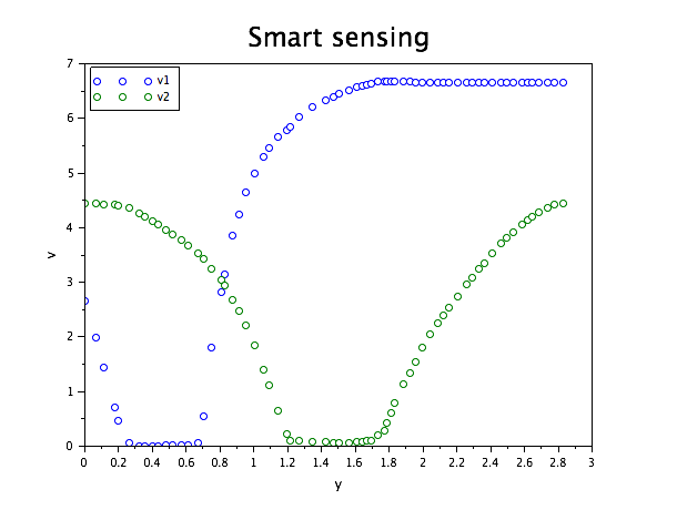
Import the data with the function fscanMat, and plot it:

BP = fscanfMat("Data/ball_p.txt");
BT = fscanfMat("Data/ball_t.txt");

Length = 67;
scf(0)
plot(BP(1:2, 1:Length)', 'o')
tutoTitle(" Smart sensing ", " y ", " v ", "v1", "v2")
//the function tutoTitle() is described in the file tutoTitle.sci

Architecture of the network & training method

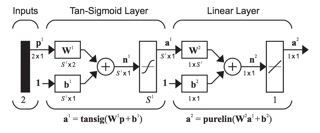
In order to get a mapping of the position of the ball, we will use a feedforward backpropagation algorithm of 10 neurons in one hidden layer. The network architecture is described as follow, with a Tan-Sigmoid activation function in the hidden layer, and a linear activation function in the output layer.

Launching the following commands, modifying the ann_FFBP_gd function in order to get the mean square errors evolution and selecting a training set of 57 measurements BP1 and BT1, keeping 10 test measurements for training assessment, we have:

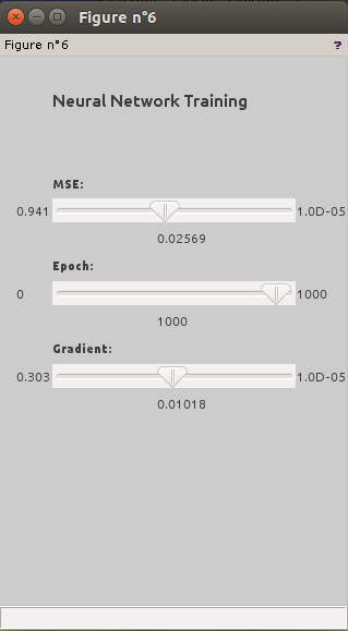
// Test data selection
K = (1:6:60)
BP_test = BP(:,K);
BT_test = BT(:,K);

// Training data selection
BP1 = BP;
BP1(:, K) = [];
BT1 = BT;
BT1(:, K) = [];

[W]=ann_FFBP_gd(BP1, BT1, [2 10 1])
//close()

Note that a second output argument MSE have to show up if you want to get the mean squared error.

Evaluation of the training quality

By modifying the function ann_FFBP_gd, we were able to get the mean squared error and plot it (that is all the beauty of open-source, you can tune everything to your need):

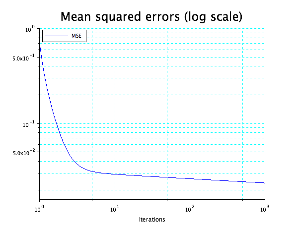
scf(2)
ind = linspace(0, 3, size(MSE, 1))
iter = 10 .^ ind;
plot2d("ll", iter, MSE, style = 2)
set(gca(), "grid", [4 4])
Titre(" Mean squared errors (log scale) ", " Iterations ", "  ", ' MSE ', ' ')

In our case, we trained the network, after 1000 epochs, the gradient of the algorithm stopped at a value of 1.018 * 10^–² , with a mean squared error (MSE) value at 2.569 * 10^-2

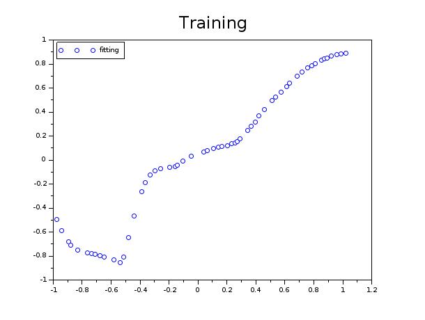
This graph represents the scatter plot of the network outputs versus targets:

Improve the quality of the training

Increasing the number of neurons and increasing the number of epochs led us to get the following training learning:

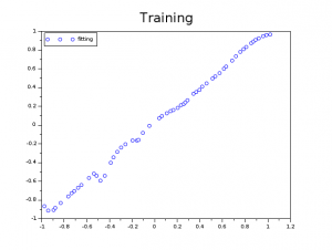
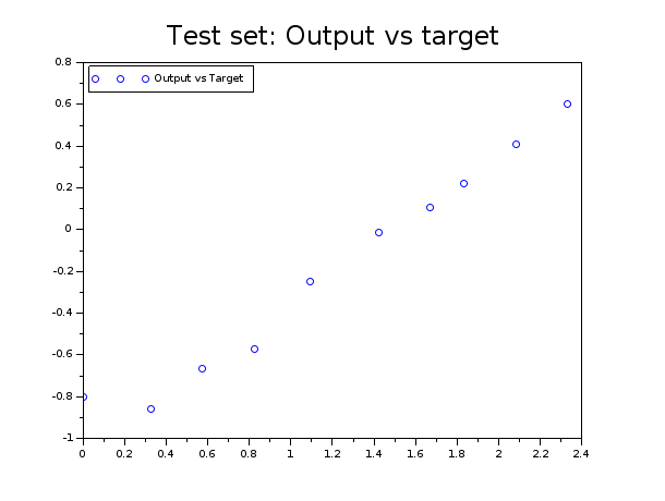
As we can appreciate, the position of the ball is much better approximated with the new settings as suggested by the test set.

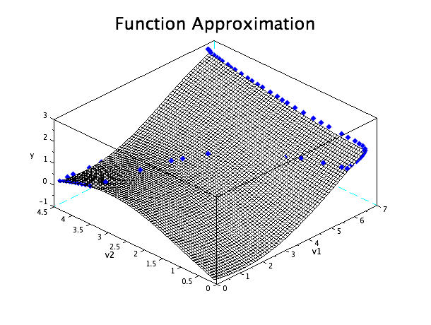
Results: approximated function

To conclude here is a representation of the function that we aimed to approximate, giving the position y of the ball depending on the voltage v1 and v2 of the solar cells: