Machine learning – Classification with SVM
The acronym SVM stands for Support Vector Machine. Given a set of training examples, each one belonging to a specific category, an SVM training algorithm creates a model that separates the categories and that can later be used to decide the category of new set of data.
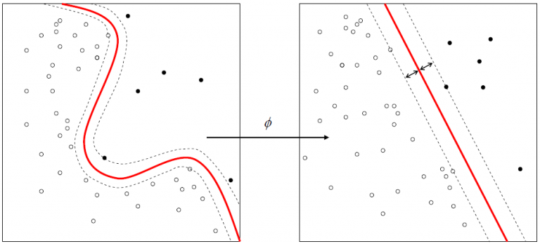
Basically, the training part consists in finding the best separating plane (with maximal margin) based on specific vector called support vector. If the decision is not feasible in the initial description space, you can increase space dimension thanks to kernel functions and may be find a hyperplane that will be your decision separator.
Scilab provides you such a tool via the libsvm toolbox. Here are some informations on the toolbox capabilities. In this tutorial, we will see together how it can be used on a specific set of data.
DataSet
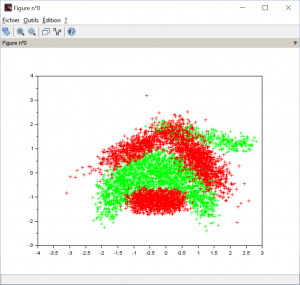
This dataset (download here) doesn’t stand for anything. It shows just a class that has a banana shape. And that is pretty cool, isn’t it? Your dataset banana.csv is made of 3 rows : x coordinate, y coordinate and class. On the above figure, green points are in class 1 and red points are in class -1. The all challenge is to find a separator that could indicate if a new data is either in the banana or not.
Model hypothesis
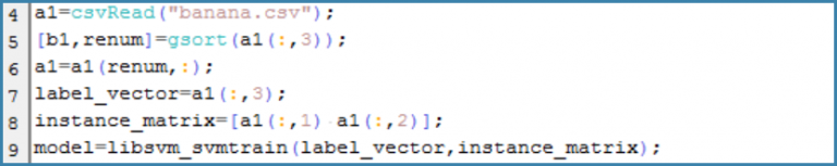
Begin with sorting your data. Thanks to gsort and renum, class 1 points will appear first. Now get your model with libsvm_svmtrain by traning it on your points (instance_matrix) and their class labels (label_vector).
Since we don’t detailed more, the model will be based on default settings. Let’s see how it is structured.
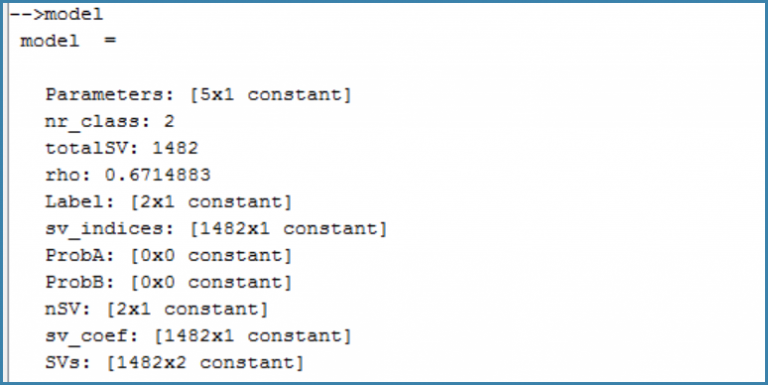
To fully understand all the informations given by the model, we invite you to read this paper on the toolbox capabilities. For the moment, we will focus on the Parameters chidren.
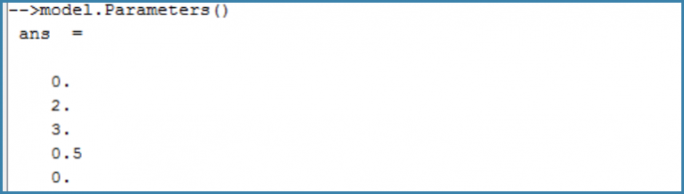
In this vector you will find :
SVM type
This toolbox provides a lot of method depending on your specific needs. In our case its a classical SVM classification as we explained it earlier. But you can use :
- 0 : C-SVC (class separation)
- 1 : Nu-SVC (nu-classification)
- 2 : One class SVM
- 3 : Epsilon-SVR (regression)
- 4 : Nu-SVR (regression)
Kernel type
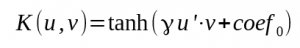
As we said, kernel function are used to increase your space dimension. Here are a few common kernel type :
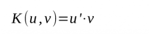
- 0 : Linear
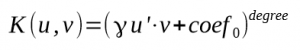
- 1 : Polynomial
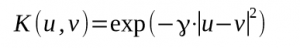
- 2 : Radial Basis Function
- 3 : Sigmoid
Kernel parameters
Last three parameters are in order degree, γ and coef0.
So, in our case we got class separation with a radial basis function as kernel. That is the default choice, but it’s sufficient for us. Actually, the radial basis kernel imply an infinite dimension. In such a space, our dataset is necessarily separable. Of course, complexity and computing time are higher but separation is ensured. If you want to try an other kernel, you can change parameters in the libsvm_svmtrain function.
Model optimization
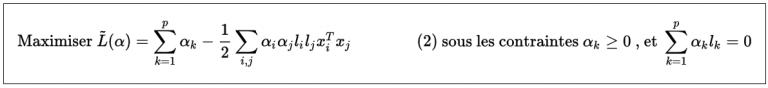
SVM optimization is an iterative process that aims to maximize the margin depending on the choosen support vectors.
When you finally got the optimal Lagrange multiplier α your decision function is now complete. The hyperplane equation can be translated in the initial descirption space thanks to the kernel function k as follow:
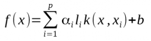
In our example, we have this:
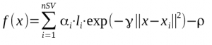
with
- nSV : Number of support vector
- αi.li = sv_coef
- xi : Support vectors SVs
- ρ = – b
As you may have noticed, those parameters appear in the model structure (see above figure). So, you are now able to build the decision function associated to your SVM trained model.
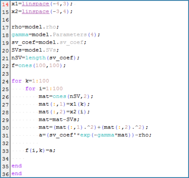
To do so, we created a grid of our description space and then with two for loops, created the f matrix of the value of the decision function on our grid following the above formula.
Visualization
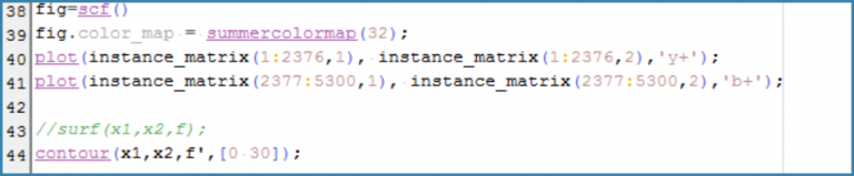
Now it’s time to see our banana separator.
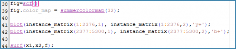
Here 2376 is the limit of class 1 data and 5300 the total length of the dataset. Thus you can assign different color to your two categories, just as we did. Our banana will be yellow (we thought it makes sense).
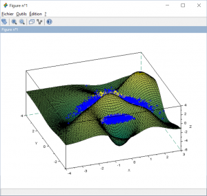
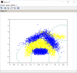
Top view of the dataset
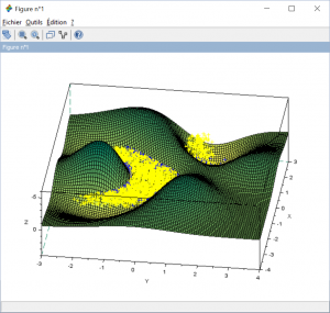
Bottom view of the dataset
Thanks to those figures, we can easily understand how the decision function works. When the decision function for a given data is positive, then this data belong to the banana class (yellow). Otherwise, it belongs to the blue class. But this visualization is not really operable. Just try the contour of the decision function on z=0.
Be careful, contour function needs f ‘ as argument and 2 level to work. Just take 0 and one far away like 30.
Conclusion
In this tutorial we show you how to train your SVM model and how to visualize your decision frontier. Now it’s time to predict!