Lagrange polynomial interpolation

This article was kindly contributed by Vlad Gladkikh

—

Assume we have data (x_i, y_i), i = 1, …, n.

The data don’t have to be equally spaced.

We can pass a Lagrange polynomial P(x) of degree n−1 through these data points.

function y = lagrange_interp(x,data)
    
    for i = 1:length(x)
        y(i) = P(x(i),data);
    end
    
endfunction

The polynomial P(x) is a linear combination of polynomials L_i(x), where each L_i(x) is of degree n−1

P(x) = y₁L₁(x) + y₂L₂(x) + … + y_nL_n(x)

The polynomials L_i(x) are defined as

L_i(x) = (x−x₁) … (x−x_i-1)(x−x_i+1) … (x−x_n) / α_i

where

α_i = (x_i−x₁) … (x_i−x_i-1)(x_i−x_i+1) … (x_i−x_n)

It is obvious that L_i(x_j) = δ_ij and therefore P(x_i) = y_i meaning that the polynomial P passes through all the data (x_i, y_i), i = 1, …, n.

If the the data (x_i, y_i) are organized in an n×2 matrix, then the polynomial P can be computed as follows

function y = P(x,data)

    n = size(data,1);

    xi = data(:,1);
    yi = data(:,2);

    L = cprod_e(xi,x) ./ cprod_i(xi); 
    y = yi' * L;

endfunction

where the function cprod_e calculates the numerators of L_i(x) for each i, namely all the products

(x−x₁) … (x−x_i-1)(x−x_i+1) … (x−x_n)

function y = cprod_e(x,a)
    
    n = length(x);
    y(1) = prod(a-x(2:$));
    for i = 2:n-1
        y(i) = prod(a-x(1:i-1))*prod(a-x(i+1:$));
    end
    y(n) = prod(a-x(1:$-1));
    
endfunction

The function cprod_i calculates all α_i for i = 1, …, n.

function y=cprod_i(x)
    
    n = length(x);
    y(1) = prod(x(1)-x(2:$));
    for i = 2:n-1
        y(i) = prod(x(i)-x(1:i-1))*prod(x(i)-x(i+1:$));
    end
    y(n) = prod(x(n)-x(1:$-1));
    
endfunction

Now, let’s test our code.

I take two examples from the book “Fundamentals of Engineering Numerical Analysis” by Prof. Parviz Moin.

Both examples use data obtained from the Runge’s function

y = 1/(1+25 x²)

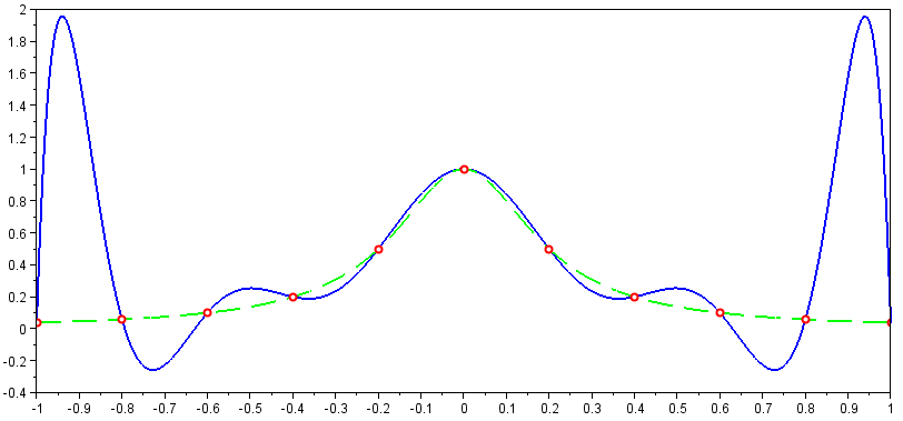
The data in the first example are equally spaced:

data1=[...
-1.0 0.038;
-0.8 0.058;
-0.6 0.1;
-0.4 0.2;
-0.2 0.5;
0.0 1.0;
0.2 0.5;
0.4 0.2;
0.6 0.1;
0.8 0.058;
1.0 0.038];

The commands to perform Lagrange interpolation are:

x = linspace(-1,1,1000);
y = lagrange_interp(x,data1);

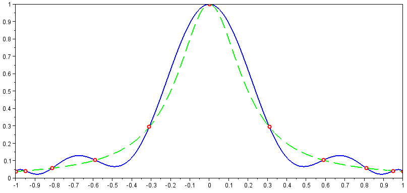
Here’s the plot of the data (red circles), the Lagrange polynomial (solid line) and the Runge’s function (dashed line):

plot(x,y,'-b',...
x, 1.0 ./ (1+25.*x.^2),'--g',...
data1(:,1),data1(:,2),'or')

The second example takes non-equally spaced data:

data2 = [...
-1.0 0.038;
-0.95 0.042;
-0.81 0.058;
-0.59 0.104;
-0.31 0.295;
0.0 1.0;
0.31 0.295;
0.59 0.104;
0.81 0.058;
0.95 0.042;
1.0 0.038];

Interpolating and plotting them as we did in the previous example produces the following picture.

y = lagrange_interp(x,data2);

plot(x,y,'-b',...
x, 1.0 ./ (1+25.*x.^2),'--g',...
data2(:,1),data2(:,2),'or')