Introduction to model reduction
Model reduction aims at providing a lighter simulation model, while describing locally with high-fidelity the behavior of the system. Starting with a finite element model, it consists in reducing the dimensionality of the solution space thus allowing faster simulation.
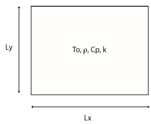
Thermal model in transient regime
We will study here the example of a thermal model of the cooling phase of a ceramic slab after an electrofusion process (see image below). You will find the code here. This tutorial is not about going into more technical details but rather to introduce you to new powerful tools and see how to move from theory to practice with Scilab. With this aim in mind, we will explain how this theory is implemented through the different Scilab functions.
Note: At any moment, you can run the all script by running main.sce.
Mesh generation
In order to create the mesh, CGLAB toolbox and plotting library are required. Thus you will be able to generate mesh following a Delaunay triangulation.
[PosNoeud, Lbord, n, tri, ech] = get_mesh (nx, ny, Lx, Ly)
This function generates a nx x ny mesh of a Lx x Ly slab. It returns absolute position of each node (PosNoeud), nodes on the edges (Lbord) and the number of nodes (n). Delaunay triangulation finaly generates the following mesh (tri).
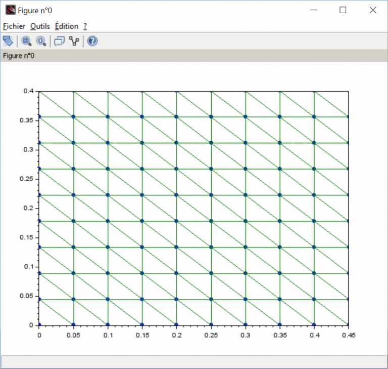
Slab modeling following a Delaunay triangulation – 100 nodes
Implementation of finite elements modeling
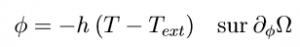
Let’s first see a classic implementation of heat transfer modeled by finite elements. h is the convection heat transfer coefficient and Text is the outside temperature.
[Q_dof, K, M] = thermique_transitoire (mu, n tri, PosNoeuds, Lbord, ech)
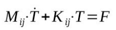
So, we wil look for the slab temperature verifying the following continuous model:

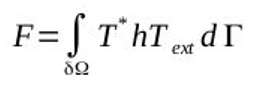
Considering a convective heat transfer on the edges,
This allows us to determine the following finite element model
|
|
|
|
|
|
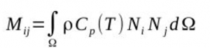
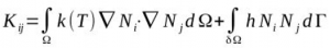
The following function’s goal is to build those matrix for every nodes.
[K, M] =assemblage (n, tri, PosNoeuds, k_th, rho, C_th)
But to do so, you will need to build your finite elements basis Ni (NEF in the code) first and compute the related Jacobian Matric ∇Nj (GEF in the code).
[we, NEF, GEF] = elemtr3dp (PosABC)
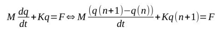
The computation is then based on an Euler implicit scheme where q(n) is the temperature at nth iteration.
Results
This computation loop gives you the temperature evolution in the ceramic slab (see animation below) and lasts a mean time of 96ms (evaluated on 100 iterations thanks to thermique_transitoire_chrono.sci).
Slab cooling computated thanks to a classic finite elements method
Model Reduction – POD method
POD stands for Proper Orthogonal Decomposition or as you may know in statistics by the name Principal Components Analysis. This method is a linear procedure that consists in creating a reduced basis for solutions built with orthogonal normal modes. Those modes, that are significant for most probable outcomes, are chosen among others thanks to a first simulation (a posteriori method).
[V_POD, erreur_POD] = POD (Q, epsilon_POD)
In the first part of this tutorial we got the temperature evolution on the whole slab over the time. A simple computation of the eigenvalues will give you the normal modes and the change of basis matrix V_POD. In order to light the model, we will keep only the significant modes defined by the epsilon_POD parameter.
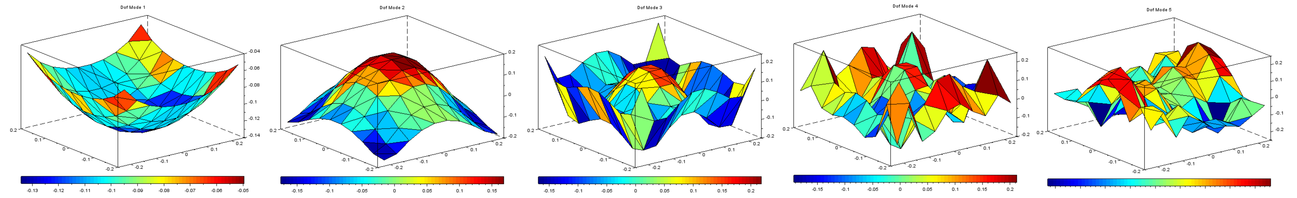
In our case, with epsilon_POD equal to 1e-3, we get 5 modes. Solutions basis is then reduced from 100 to 5 vectors with accuracy in range of 5,8e-4.

5 modes significant for the temperature evolution
[] = thermiPOD (K, M, P, tri, PosNoeuds, Lbord)
The computation is the same as you have seen previously, using the same Euler implicit Scheme transposed in reduced basis:
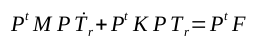
|
With Tr the temperatue in the reduced basis and P the change of basis matrix: |

|
Results
This computation loop gives you a pretty accurate approximation of the temperature evolution in the ceramic slab (see animation below) and lasts a mean time of 3ms (evaluated on 100 iterations thanks to thermiquePOD_chrono.sci). It is 30 times faster than a classic finite elements solving.
Slab cooling computated thanks to a reduced model (POD)
Conclusion
Even for such a little mesh (100 nodes), computation time optimization is significant (30 times faster). Setting an efficient Design of Experiment (DoE) would allow to perform high-fidelity interpolation between two simulations, enabling design space exploration and multi-objective optimization.