Famous Datasets
The atoms toolbox rdataset provides a collection of 761 datasets that were originally distributed alongside R.
Download it on ATOMS:
https://atoms.scilab.org/toolboxes/rdataset
Collaborate to the code on our Forge:
https://forge.scilab.org/index.php/p/rdataset/
You can import easily those famous dataset, and get inspiration from the open source software R, specialized in statistics.
93 Cars on Sale in the USA in 1993
// Read the dataset Cars93 from MASS
[data,desc] = rdataset_read("MASS","Cars93");
// read description
disp(desc)
// read header of data
disp(data(1))
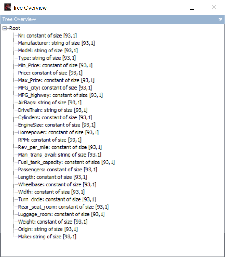
//view the hierarchy of data as a tree
tree_show(data)
//store as matrix of string
M=[]
for i=2:29
    M=[M,string(data(i))]
end

//add header
M=[data(1)(2:29);M]

//export as CSV
csvWrite(M,"Cars93.csv")
|
Package |
Item |
Title |
Rows |
Cols |
has_logical |
has_binary |
has_numeric |
has_character |
CSV |
Doc |
|
MASS |
Cars93 |
Data from 93 Cars on Sale in the USA in 1993 |
93 |
27 |
FALSE |
TRUE |
TRUE |
FALSE |
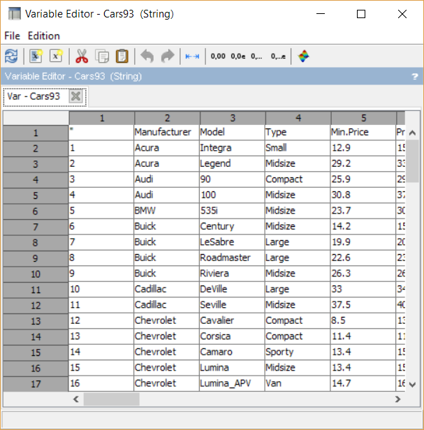
You can also import the data in a more classic way after downloading it above:
Cars93 = csvRead('Cars93.csv',',','.', 'string');

D=csvRead('Cars93.csv'); data = D(2:$,:);
This enables to have a single matrix containing all data in our variable workspace:
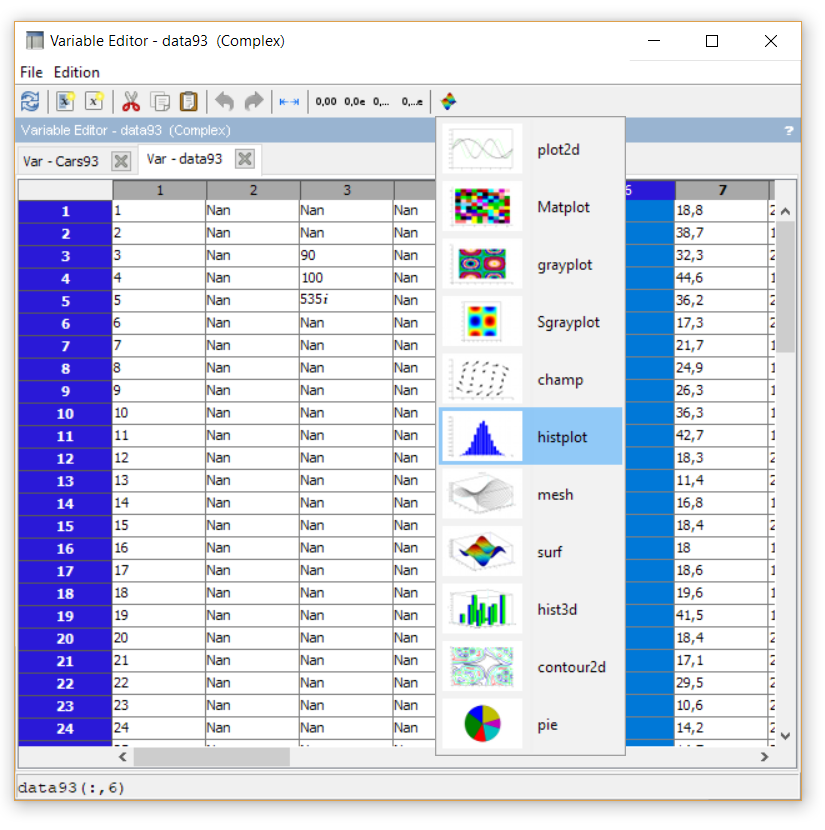
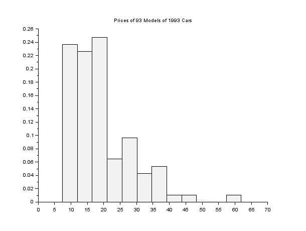
The first distribution of interest would be the price of the different models:
histplot(12,data(:,6))

title("Prices of 93 Models of 1993 Cars")
One way to represent data relatively is a pie chart:
Cars93(2:$,4)

m=tabul(Cars93(2:$,4))

pie(m(2),m(1))

pie(m(2));legend(m(1));
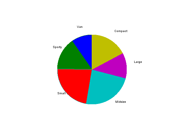
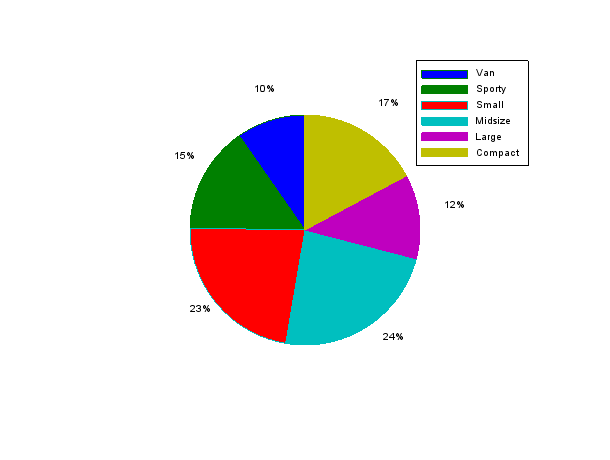
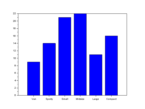
Some might advocate that it is easier to differentiate the respective value of categories when plotted on the same scale.
For that, a bar chart is more appropriate. However, you need to change the ticks labels to have a representation of non-numeric categories.
//Bar

bar(m(2));

h = get("current_entity");

h.parent.x_ticks.labels = m(1)
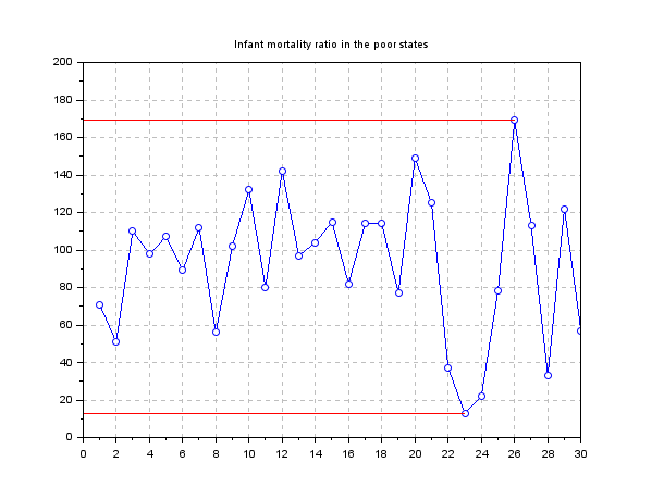
The Wealth of Nations
Another interesting dataset to look at is considering the United Nations (1998) Social indicators: infant mortality and Gross domestic product(GDP)
// Read the dataset survey from from UN

[data,desc] = rdataset_read("car","UN");

// read description

disp(desc)

// read header of data

disp(data(1))
Some data might not be defined (NaN = Not a Number) in our dataset, so we can use the function thrownan.
// History plot

// Getting rid of the NaN entries

[gdp,k] = thrownan(data.gdp);

[rationonan,kk] = thrownan(data.infant_mortality(k));

gdpnonan = gdp(kk);
// Plot

[p,i] = gsort(gdpnonan,'g','i');

scf(1); clf(1);

plot([1:30],rationonan(i(1:30)),'bo-')

plot([1:30],data(k(kk(i(1:30))),15),'go-')

[m,im] = min(rationonan(i(1:30)));

plot([0,im],[m,m],'r')

[M,iM] = max(rationonan(i(1:30)));

plot([0,iM],[M,M],'r')

set(gca(),"grid",[1 1]*color('gray'));

set(gca(),"data_bounds",[0 30 0 200]);

title('Infant mortality ratio in the poor states');
Now let's look at a Pareto chart:
// Bar Chart and cumulative

[gdpnonan,i] = thrownan(data.gdp);

[gdp,j] = gsort(gdpnonan);

tot_gdp = sum(gdp);

cum_gdp = cumsum(gdp(1:10));

scf(4); clf(4);

bar(gdp(1:10)*100/tot_gdp)

plot([1:10],cum_gdp*100/tot_gdp,'ro-')

set(gca(),"grid",[1 1]*color('gray'));
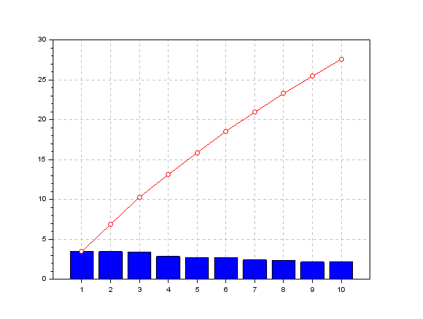
We have plotted the percentage of the global per capita GDP for the 10 states with highest per capita GDP, while the red line shows the cumulative sum of these values: it points out that these 10 states cover the 30% of the global per capita GDP...
You can find more on this tutorial from Openeering on Data mining.
Hot dogs and buns
Another way to find data is to crawl the internet. For instance you find tremendous sources of wisdom, such as this great proof of cultural domination from the US: Nathan's Hot Dog Eating Contest
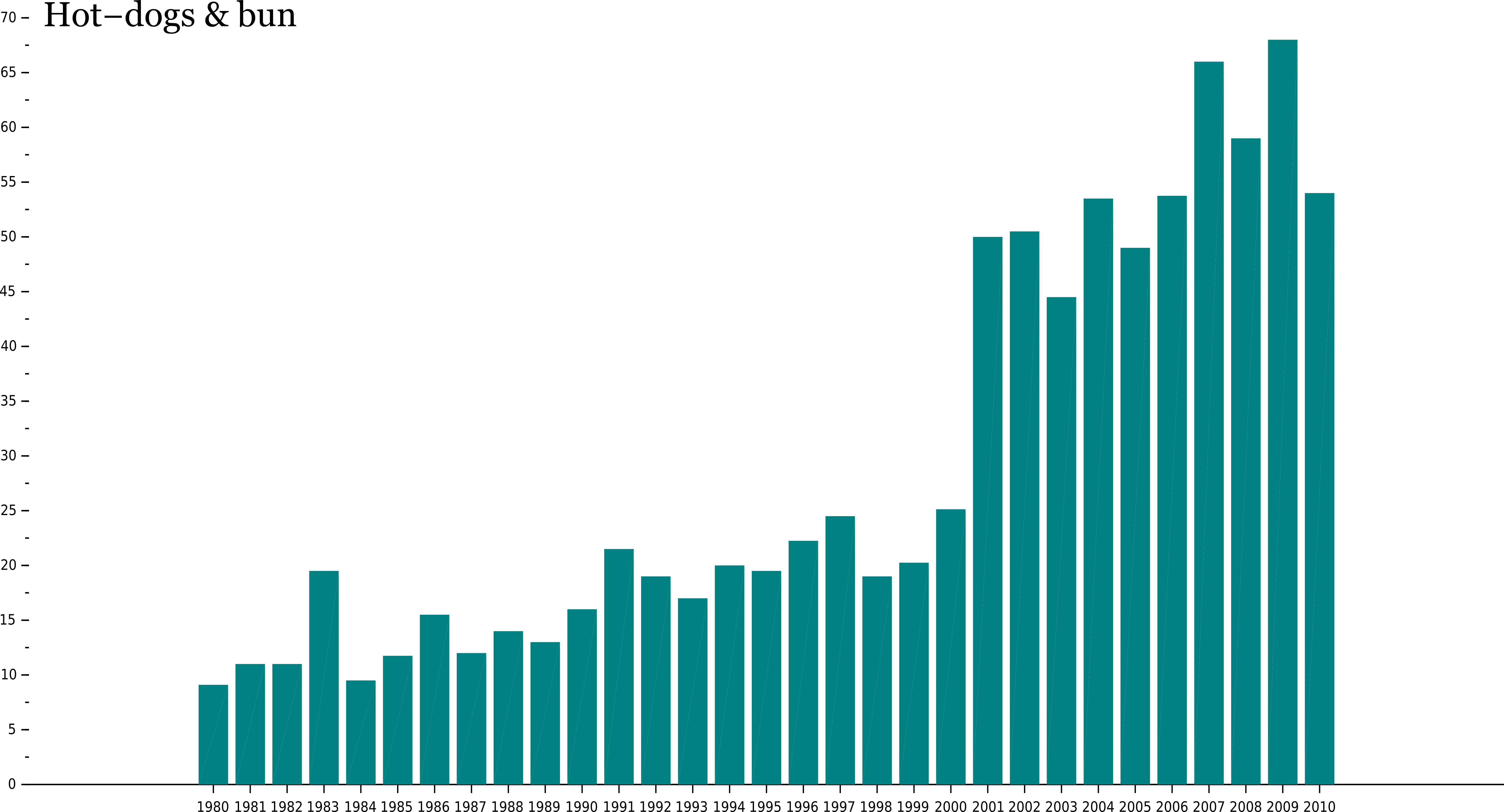
This graphic was produced with Scilab, exported as a vectorial format SVG, and edited with the open-source software Inkscape.
We could dedicated a full tutorial to this subject, but let us shortly go through the basics:
First we can download the content of the webpage with the function getURL:
--> filename=getURL("en.wikipedia.org/wiki/Nathan%27s_Hot_Dog_Eating_Contest")
 filename  =

 C:\myFolder\Nathan's_Hot_Dog_Eating_Contest
Then we can real the HTML, with the function we use in Scilab for XML, such as xmlRead:
--> doc=xmlRead(filename)
 doc  =

XML Document
url: file:///C:/myFolder/Nathan's_Hot_Dog_Eating_Contest
root: XML Element
We need to know a little bit about HTML in order to find the data we are looking for:
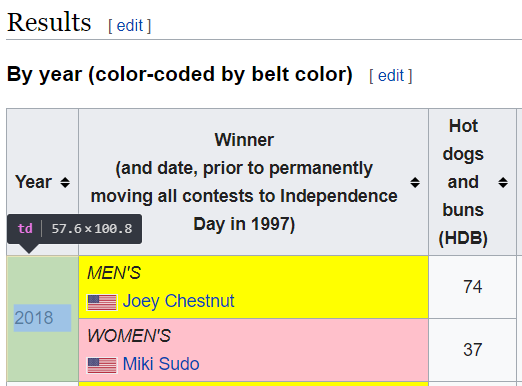
You can inspect the webpages in your browser (Ctrl+Maj+I with Chrome).
Extracting the nodes corresponding to the lines of a table in html would be performed thanks to the function xmlXPath:
--> td=xmlXPath(doc, "//td")
 td  =

XML List
size: 367
We find 367 occurencies. By browsing, we finally find the content we are looking for:
--> td(10).content
 ans  =

 2018
You can write a program based on this principal to extract valuable data from webpages. Enjoy hacking ;)