Blending Some Control Engineering Flavor

This content was kindly contributed by Dew Toochinda, the Scilab Ninja, and originally posted on https://scilabdotninja.wordpress.com/

 

Download the files for this tutorial:

So, let’s discuss some common task for control system analysis and design. It is suitable for an introductory document to limit the scope to only Linear Time-Invariant (LTF) systems, such that the plant and controller can be described as transfer functions in the Laplace domain (continuous-time), or the Z-domain (discrete-time). We also consider only Single-Input-Single-Output (SISO) systems.

Transfer Function Representation

An LTI plant can be modeled from physics using differential equation mathematics, then converted to a transfer function by Laplace transform. This is where we start our discussion. Given a plant represented by

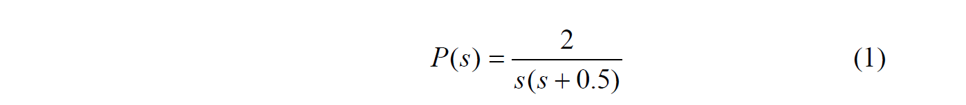
which is a simplified example of permanent magnet DC motor. To construct this plant in Scilab workspace, start with a seed s representing Laplace variable.

--> s=poly(0,'s')
 s  = 

    
   s

Then we can build on s any polynomial or rational function. For (1),

--> P = 2/(s*(s+0.5))
 P  = 

              
      2       
   ---------  
           2  
   0.5s + s   

Those who are familiar with MATLAB may notice that the power of s is displayed in reverse fashion in Scilab; i.e., starting from lowest order term. You somehow have to get used to this, especially when representing the numerator and denominator in vector form.

At this point, our plant appears like a rational function , but is not yet a linear transfer function that Scilab could interpret. We need to do one more step by using syslin command

--> P = syslin('c',P)
 P  = 

              
      2       
   ---------  
           2  
   0.5s + s  

We do this in two steps to make it clear. Next time you can save time by generating a transfer function in one step.

Now we can observe Bode frequency response of P

--> bode(P)

which yields Figure 1.

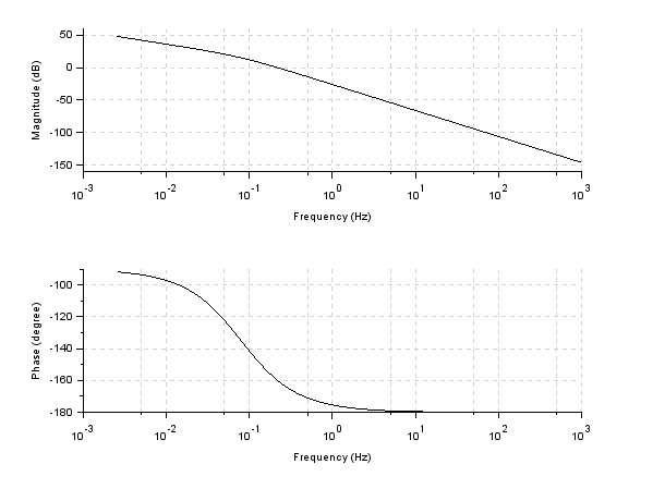
Figure 1 Bode plot of P(s)

 

Some other useful commands that you can try by your own

nyquist(P) : generate a Nyquist plot

plzr(P): plot pole/zero mapping in complex plane

 

Now, we can do standard computation with transfer functions in Scilab. Say, suppose we have a controller

Construct it in Scilab
--> C=syslin('c',(s+1)/(s+10))
 C  = 

            
   1 + s    
   -------  
            
   10 + s   

To compute a loop transfer function L(s) = C(s)P(s)

--> L = C*P
 L  = 

                    
       2 + 2s       
   ---------------  
             2   3  
   5s + 10.5s + s   

Likewise, for the sensitivity S(s) = 1/(1+L(s)) and complementary sensitivity T(s) = L(s)/(1+L(s))

--> S = 1/(1+L)
 S  = 

               2   3    
     5s + 10.5s + s     
   -------------------  
                 2   3  
   2 + 7s + 10.5s + s   

--> T = L/(1+L)
 T  = 

                        
         2 + 2s         
   -------------------  
                 2   3  
   2 + 7s + 10.5s + s   

Stability of closed-loop system can be determined from the poles of S or T. That raises a question. How to compute the pole of a transfer function?

The way I used to get around is to convert the data to state-space format, say, for T(s)

--> Tss = tf2ss(T);

Then we can check the eigenvalue of matrix A in Tss by command spec

--> spec(Tss.A)
 ans  =

  -9.8070205  
  -0.3464898 + 0.2896211i
  -0.3464898 - 0.2896211i

Since all poles have negative real parts, this feedback system is stable

A finished zcos file is available for download below, but I recommend that you try building one by your own first to clearly understand the process.

Connect the diagram as shown in Figure 2. The black and red signal routes cannot be mixed. Here we have red line only to the scope representing simulation clock. It is a good practice to label the blocks and signals with TEXT_f so that your diagram is understandable to others, but not required for the simulation to work.

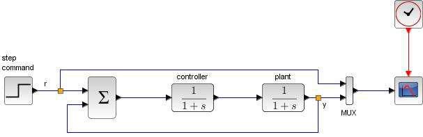
Figure 2 feedback structure for simulation

 

Save the diagram to myfeedback.zcos, or whatever name you like.

Note that the CLR block has defaulted data 1/(1+s). We must put in data for our controller and plant. Figure 2 shows a CLR block after we double-click to input data

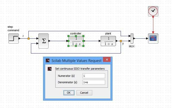
Figure 3 parameter window of CLR block

This poses another problem. The CLR block needs data in the form of numerator and denominator polynomials, but we have in Scilab workspace transfer functions C and P. For example,

--> P.num
 ans  =

    
   2

--> P.den
 ans  =

          2
   0.5s +s 

So we simply put C.num, C.den and P.num, P.den into the controller and plant CLR blocks, respectively, as shown in Figure 4.

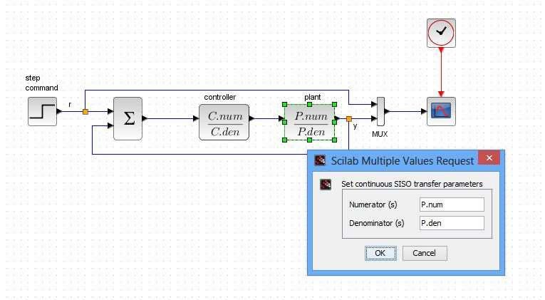
Figure 4 putting plant and controller data into CLR blocks

We’re almost done. The rest is just trivial task like setting simulation and scope parameters. You might not get good values at start, especially when this controller does not come from a design spec. We have no idea on its performance. Try adjusting the Y-axis range of scope to Ymin = 0, Ymax = 2. Set final integration time = 30 (and set the scope Refresh period to match). Run the simulation and see what happens then readjust them.

The resulting response is unstable. Can you figure out what goes wrong?

It turns out that we forget to set minus sign for the feedback path. Doule-click on the summing junction block to open its parameter window. Change the vector value in Inputs ports signs/gain field from [1; 1] to [1, -1]. The block now shows minus sign for the feedback.

Run the simulation again. You should now see the step response in Figure 5.

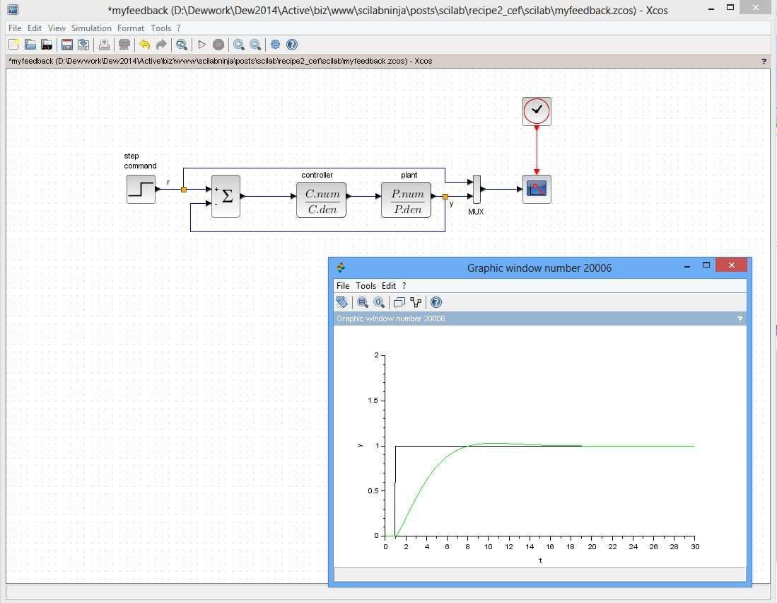
Figure 5 step response from the simulation

Bravo! Now you have some basics of Scilab and Xcos to get started on using them on a more challenged problem. To learn more, the Scilab Control Engineering Basics on our website might be helpful.

 

Exercise

 

1. Change the controller block in myfeedback.zcos to a PID block (in Continuous time systems palette). Double-click the block to adjust PID gains and run the simulation. Could you get a better response with some choice of PID gains?